Scope

In this post, we use early stopping to reduce overfitting when training an XGBoost model. We start with a short recap on early stopping and overfitting. After that, we use the early stopping mechanism of XGBoost and train a model on the Spam Classification data set. Finally we show how to simultaneously tune hyperparameters and use early stopping. The reader should be familiar with tuning in the mlr3 ecosystem.

Early Stopping

Early stopping is a technique used to reduce overfitting when fitting a model in an iterative process. Overfitting occurs when a model fits increasingly to the training data but the performance on unseen data decreases. This means the model’s training error decreases, while its test performance deteriorates. When using early stopping, the performance is monitored on a test set, and the training stops when performance decreases in a specific number of iterations.

XGBoost with Early Stopping

We initialize the random number generator with a fixed seed for reproducibility. The mlr3verse package provides all functions required for this example.

set.seed(7832)

library(mlr3verse)

When training an XGBoost model, we can use early stopping to find the optimal number of boosting rounds. The partition() function splits the observations of the task into two disjoint sets. We use 80% of observations to train the model and the remaining 20% as the test set to monitor the performance.

task = tsk("spam")
split = partition(task, ratio = 0.8)
task$set_row_roles(split$test, "test")

The early_stopping_set parameter controls which set is used to monitor the performance. Additionally, we need to define the range in which the performance must increase with early_stopping_rounds and the maximum number of boosting rounds with nrounds. In this example, the training is stopped when the classification error is not decreasing for 100 rounds or 1000 rounds are reached.

learner = lrn("classif.xgboost",
  nrounds = 1000,
  early_stopping_rounds = 100,
  early_stopping_set = "test",
  eval_metric = "error"
)

We train the learner with early stopping.

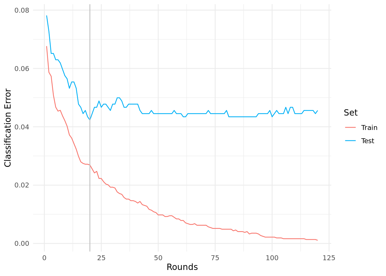
learner$train(task)

The $evaluation_log of the model stores the performance scores on the training and test set. Figure 1 shows that the classification error on the training set decreases, whereas the error on the test set increases after 20 rounds.

Code

library(ggplot2)
library(data.table)

data = melt(
  learner$model$evaluation_log,
  id.vars = "iter",
  variable.name = "set",
  value.name = "error"
)

ggplot(data, aes(x = iter, y = error, group = set)) +
  geom_line(aes(color = set)) +
  geom_vline(aes(xintercept = learner$model$best_iteration), color = "grey") +
  scale_colour_manual(values=c("#f8766d", "#00b0f6"), labels = c("Train", "Test")) +
  labs(x = "Rounds", y = "Classification Error", color = "Set") +
  theme_minimal()

Comparison between train and test set classification error.

The slot $best_iteration contains the optimal number of boosting rounds.

learner$model$best_iteration

[1] 20

Note that, learner$predict() will use the model from the last iteration, not the best one. See the next section on how to fit a model with the optimal number of boosting rounds and hyperparameter configuration.

Tuning

In this section, we want to tune the hyperparameters of an XGBoost model and find the optimal number of boosting rounds in one go. For this, we need the early stopping callback which handles early stopping during the tuning process. The performance of a hyperparameter configuration is evaluated with a resampling strategy while tuning e.g. 3-fold cross-validation. In each resampling iteration, a new XGBoost model is trained and early stopping is used to find the optimal number of boosting rounds. This results in three different optimal numbers of boosting rounds for one hyperparameter configuration when applying 3-fold cross-validation. The callback picks the maximum of the three values and writes it to the archive. It uses the maximum value because the final model is fitted on the complete data set. Now let’s start with a practical example.

First, we load the XGBoost learner and set the early stopping parameters.

learner = lrn("classif.xgboost",
  nrounds = 1000,
  early_stopping_rounds = 100,
  early_stopping_set = "test"
)

Next, we load a predefined tuning space from the mlr3tuningspaces package. The tuning space includes the most commonly tuned parameters of XGBoost.

tuning_space = lts("classif.xgboost.default")
as.data.table(tuning_space)

                  id lower upper logscale
1:               eta 1e-04     1     TRUE
2:           nrounds 1e+00  5000    FALSE
3:         max_depth 1e+00    20    FALSE
4:  colsample_bytree 1e-01     1    FALSE
5: colsample_bylevel 1e-01     1    FALSE
6:            lambda 1e-03  1000     TRUE
7:             alpha 1e-03  1000     TRUE
8:         subsample 1e-01     1    FALSE

We argument the learner with the tuning space.

learner = lts(learner)

The default tuning space contains the nrounds hyperparameter. We have to overwrite it with an upper bound for early stopping.

learner$param_set$set_values(nrounds = 1000)

We run a small batch of random hyperparameter configurations.

instance = tune(
  tuner = tnr("random_search", batch_size = 2),
  task = task,
  learner = learner,
  resampling = rsmp("cv", folds = 3),
  measure = msr("classif.ce"),
  term_evals = 4,
  callbacks = clbk("mlr3tuning.early_stopping")
)

We can see that the optimal number of boosting rounds (max_nrounds) strongly depends on the other hyperparameters.

as.data.table(instance$archive)[, list(batch_nr, max_nrounds, eta, max_depth, colsample_bytree, colsample_bylevel, lambda, alpha, subsample)]

   batch_nr max_nrounds       eta max_depth colsample_bytree colsample_bylevel     lambda     alpha subsample
1:        1        1000 -4.129996        13        0.5466492         0.3051989 -0.9448420  2.535477 0.5454539
2:        1         998 -3.338899         8        0.6193478         0.7392354 -2.2338126  1.793921 0.2294161
3:        2        1000 -6.059897         5        0.6118892         0.5445475 -6.5698270  5.414224 0.9635730
4:        2        1000 -4.528129         1        0.1094186         0.2526143 -0.7535105 -3.041829 0.5934376

In the best hyperparameter configuration, the value of nrounds is replaced by max_nrounds and early stopping is deactivated.

instance$result_learner_param_vals

$nrounds
[1] 998

$nthread
[1] 1

$verbose
[1] 0

$early_stopping_set
[1] "none"

$eta
[1] 0.03547598

$max_depth
[1] 8

$colsample_bytree
[1] 0.6193478

$colsample_bylevel
[1] 0.7392354

$lambda
[1] 0.1071192

$alpha
[1] 6.012984

$subsample
[1] 0.2294161

Finally, fit the final model on the complete data set.

learner = lrn("classif.xgboost")
learner$param_set$values = instance$result_learner_param_vals
learner$train(task)

The trained model can now be used to make predictions on new data.

We can also use the AutoTuner to get a tuned XGBoost model. Note that, early stopping is deactivated when the final model is fitted.