Scope

The predictive performance of modern machine learning algorithms is highly dependent on the choice of their hyperparameter configuration. Options for setting hyperparameters are tuning, manual selection by the user, and using the default configuration of the algorithm. The default configurations are chosen to work with a wide range of data sets but they usually do not achieve the best predictive performance. When tuning a learner in mlr3, we can run the default configuration as a baseline. Seeing how well it performs will tell us whether tuning pays off. If the optimized configurations perform worse, we could expand the search space or try a different optimization algorithm. Of course, it could also be that tuning on the given data set is simply not worth it.

Probst et al. (2019) studied the tunability of machine learning algorithms. They found that the tunability of algorithms varies widely. Algorithms like glmnet and XGBoost are highly tunable, while algorithms like random forests work well with their default configuration. The highly tunable algorithms should thus beat their baselines more easily with optimized hyperparameters. In this article, we will tune the hyperparameters of a random forest and compare the performance of the default configuration with the optimized configurations.

Example

We tune the hyperparameters of the ranger learner on the spam data set. The search space is taken from Bischl et al. (2021).

library(mlr3tuning)
library(mlr3learners)

learner = lrn("classif.ranger",
  mtry.ratio      = to_tune(0, 1),
  replace         = to_tune(),
  sample.fraction = to_tune(1e-1, 1),
  num.trees       = to_tune(1, 2000)
)

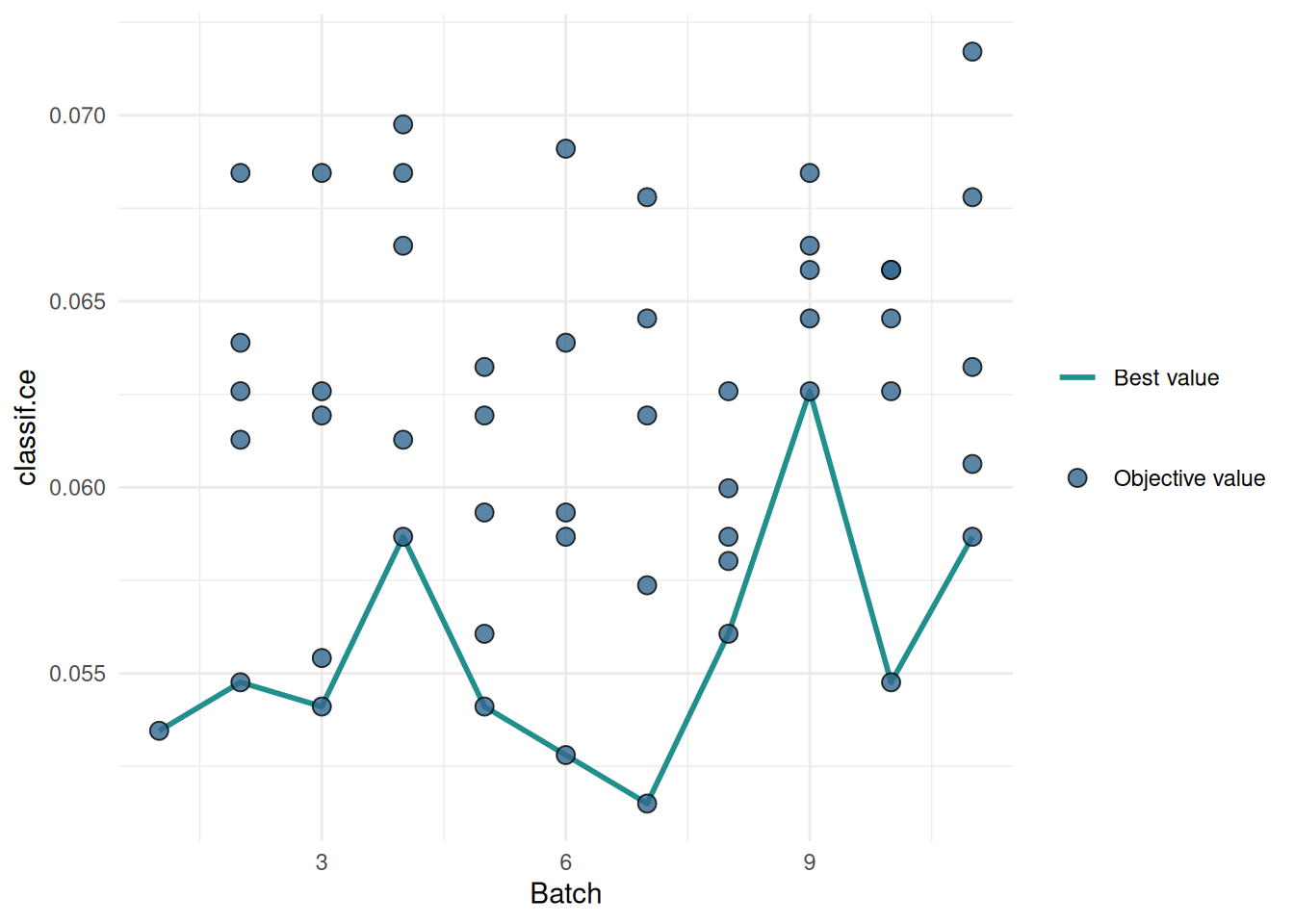
When creating the tuning instance, we pass the mlr3tuning.default_configuration callback to test the default hyperparameter configuration. The default configuration is evaluated in the first batch of the tuning run. The other batches use the specified tuning method. In this example, they are randomly drawn configurations.

instance = tune(
  tuner = tnr("random_search", batch_size = 5),
  task = tsk("spam"),
  learner = learner,
  resampling = rsmp ("holdout"),
  measures = msr("classif.ce"),
  term_evals = 51,
  callbacks = clbk("mlr3tuning.default_configuration")
)

The default configuration is recorded in the first row of the archive. The other rows contain the results of the random search.

as.data.table(instance$archive)[, .(batch_nr, mtry.ratio, replace, sample.fraction, num.trees, classif.ce)]

    batch_nr mtry.ratio replace sample.fraction num.trees classif.ce
 1:        1  0.1228070    TRUE       1.0000000       500 0.05345502
 2:        2  0.3501304   FALSE       0.7508930      1333 0.05475880
 3:        2  0.6235093   FALSE       0.3830663       682 0.06388527
 4:        2  0.8002110   FALSE       0.8686475       466 0.06127771
 5:        2  0.2390842    TRUE       0.4383263      1081 0.06258149
---                                                                 
47:       11  0.2220490    TRUE       0.3372232       486 0.06062581
48:       11  0.9806011   FALSE       0.6418448       773 0.06323338
49:       11  0.8375713   FALSE       0.2742567      1964 0.06779661
50:       11  0.9514603   FALSE       0.9537379       626 0.07170795
51:       11  0.8203689   FALSE       0.8481546       295 0.05867014

We plot the performances of the evaluated hyperparameter configurations. The blue line connects the best configuration of each batch. We see that the default configuration already performs well and the optimized configurations can not beat it.

library(mlr3viz)

autoplot(instance, type = "performance")

Conlcusion

The time required to test the default configuration is negligible compared to the time required to run the hyperparameter optimization. It gives us a valuable indication of whether our tuning is properly configured. Running the default configuration as a baseline is a good practice that should be used in every tuning run.

Session Information

sessioninfo::session_info(info = "packages")

═ Session info ═══════════════════════════════════════════════════════════════════════════════════════════════════════
─ Packages ───────────────────────────────────────────────────────────────────────────────────────────────────────────
 package        * version    date (UTC) lib source
 backports        1.5.0      2024-05-23 [1] RSPM
 bbotk            1.8.1      2025-11-26 [1] RSPM
 checkmate        2.3.4      2026-02-03 [1] RSPM
 cli              3.6.5      2025-04-23 [1] RSPM
 codetools        0.2-20     2024-03-31 [2] CRAN (R 4.5.2)
 crayon           1.5.3      2024-06-20 [1] RSPM
 data.table     * 1.18.2.1   2026-01-27 [1] RSPM
 digest           0.6.39     2025-11-19 [1] RSPM
 dplyr            1.2.0      2026-02-03 [1] RSPM
 evaluate         1.0.5      2025-08-27 [1] RSPM
 farver           2.1.2      2024-05-13 [1] RSPM
 fastmap          1.2.0      2024-05-15 [1] RSPM
 future           1.69.0     2026-01-16 [1] RSPM
 future.apply     1.20.2     2026-02-20 [1] RSPM
 generics         0.1.4      2025-05-09 [1] RSPM
 ggplot2          4.0.2      2026-02-03 [1] RSPM
 globals          0.19.0     2026-02-02 [1] RSPM
 glue             1.8.0      2024-09-30 [1] RSPM
 gridExtra        2.3        2017-09-09 [1] RSPM
 gtable           0.3.6      2024-10-25 [1] RSPM
 htmltools        0.5.9      2025-12-04 [1] RSPM
 htmlwidgets      1.6.4      2023-12-06 [1] RSPM
 jsonlite         2.0.0      2025-03-27 [1] RSPM
 knitr            1.51       2025-12-20 [1] RSPM
 labeling         0.4.3      2023-08-29 [1] RSPM
 lattice          0.22-7     2025-04-02 [2] CRAN (R 4.5.2)
 lgr              0.5.2      2026-01-30 [1] RSPM
 lifecycle        1.0.5      2026-01-08 [1] RSPM
 listenv          0.10.0     2025-11-02 [1] RSPM
 magrittr         2.0.4      2025-09-12 [1] RSPM
 Matrix           1.7-4      2025-08-28 [2] CRAN (R 4.5.2)
 mlr3           * 1.4.0      2026-02-19 [1] RSPM
 mlr3learners   * 0.14.0     2025-12-13 [1] RSPM
 mlr3measures     1.2.0      2025-11-25 [1] RSPM
 mlr3misc         0.21.0     2026-02-26 [1] RSPM
 mlr3tuning     * 1.5.1      2025-12-14 [1] RSPM
 mlr3viz        * 0.11.0     2026-02-22 [1] RSPM
 mlr3website    * 0.0.0.9000 2026-02-27 [1] Github (mlr-org/mlr3website@f6e32a7)
 otel             0.2.0      2025-08-29 [1] RSPM
 palmerpenguins   0.1.1      2022-08-15 [1] RSPM
 paradox        * 1.0.1      2024-07-09 [1] RSPM
 parallelly       1.46.1     2026-01-08 [1] RSPM
 pillar           1.11.1     2025-09-17 [1] RSPM
 pkgconfig        2.0.3      2019-09-22 [1] RSPM
 R6               2.6.1      2025-02-15 [1] RSPM
 ranger           0.18.0     2026-01-16 [1] RSPM
 RColorBrewer     1.1-3      2022-04-03 [1] RSPM
 Rcpp             1.1.1      2026-01-10 [1] RSPM
 rlang            1.1.7      2026-01-09 [1] RSPM
 rmarkdown        2.30       2025-09-28 [1] RSPM
 S7               0.2.1      2025-11-14 [1] RSPM
 scales           1.4.0      2025-04-24 [1] RSPM
 sessioninfo      1.2.3      2025-02-05 [1] RSPM
 stringi          1.8.7      2025-03-27 [1] RSPM
 tibble           3.3.1      2026-01-11 [1] RSPM
 tidyselect       1.2.1      2024-03-11 [1] RSPM
 uuid             1.2-2      2026-01-23 [1] RSPM
 vctrs            0.7.1      2026-01-23 [1] RSPM
 viridis          0.6.5      2024-01-29 [1] RSPM
 viridisLite      0.4.3      2026-02-04 [1] RSPM
 withr            3.0.2      2024-10-28 [1] RSPM
 xfun             0.56       2026-01-18 [1] RSPM
 yaml             2.3.12     2025-12-10 [1] RSPM

 [1] /usr/local/lib/R/site-library
 [2] /usr/local/lib/R/library
 * ── Packages attached to the search path.

──────────────────────────────────────────────────────────────────────────────────────────────────────────────────────

References

Bischl, Bernd, Martin Binder, Michel Lang, et al. 2021. “Hyperparameter Optimization: Foundations, Algorithms, Best Practices and Open Challenges.” arXiv:2107.05847 [Cs, Stat], July. http://arxiv.org/abs/2107.05847.

Probst, Philipp, Anne-Laure Boulesteix, and Bernd Bischl. 2019. “Tunability: Importance of Hyperparameters of Machine Learning Algorithms.” Journal of Machine Learning Research 20 (53): 1–32. http://jmlr.org/papers/v20/18-444.html.