Intro

This is the second part of a serial of tutorials. The other parts of this series can be found here:

We will continue working with the German credit dataset. In Part I, we peeked into the dataset by using and comparing some learners with their default parameters. We will now see how to:

Tune hyperparameters for a given problem
Perform nested resampling

Prerequisites

First, load the packages we are going to use:

library("mlr3verse")
library("data.table")
library("mlr3tuning")
library("ggplot2")

We initialize the random number generator with a fixed seed for reproducibility, and decrease the verbosity of the logger to keep the output clearly represented.

set.seed(7832)
lgr::get_logger("mlr3")$set_threshold("warn")
lgr::get_logger("bbotk")$set_threshold("warn")

We use the same Task as in Part I:

task = tsk("german_credit")

We also might want to use multiple cores to reduce long run times of tuning runs.

future::plan("multiprocess")

Evaluation

We will evaluate all hyperparameter configurations using 10-fold cross-validation. We use a fixed train-test split, i.e. the same splits for each evaluation. Otherwise, some evaluation could get unusually “hard” splits, which would make comparisons unfair.

cv10 = rsmp("cv", folds = 10)

# fix the train-test splits using the $instantiate() method
cv10$instantiate(task)

# have a look at the test set instances per fold
cv10$instance

      row_id fold
   1:     18    1
   2:     19    1
   3:     35    1
   4:     38    1
   5:     55    1
  ---            
 996:    973   10
 997:    975   10
 998:    981   10
 999:    993   10
1000:    998   10

Simple Parameter Tuning

Parameter tuning in mlr3 needs two packages:

The paradox package is used for the search space definition of the hyperparameters.
The mlr3tuning package is used for tuning the hyperparameters.

The packages are loaded by the mlr3verse package.

Search Space and Problem Definition

First, we need to decide what Learner we want to optimize. We will use LearnerClassifKKNN, the “kernelized” k-nearest neighbor classifier. We will use kknn as a normal kNN without weighting first (i.e., using the rectangular kernel):

knn = lrn("classif.kknn", predict_type = "prob", kernel = "rectangular")

As a next step, we decide what parameters we optimize over. Before that, though, we are interested in the parameter set on which we could tune:

knn$param_set

            id    class lower upper nlevels
1:           k ParamInt     1   Inf     Inf
2:    distance ParamDbl     0   Inf     Inf
3:      kernel ParamFct    NA    NA      10
4:       scale ParamLgl    NA    NA       2
5:     ykernel ParamUty    NA    NA     Inf
6: store_model ParamLgl    NA    NA       2

We first tune the k parameter (i.e. the number of nearest neighbors), between 3 to 20. Second, we tune the distance function, allowing L1 and L2 distances. To do so, we use the paradox package to define a search space (see the online vignette for a more complete introduction.

search_space = ps(
  k = p_int(3, 20),
  distance = p_int(1, 2)
)

As a next step, we define a TuningInstanceSingleCrit that represents the problem we are trying to optimize.

instance_grid = TuningInstanceSingleCrit$new(
  task = task,
  learner = knn,
  resampling = cv10,
  measure = msr("classif.ce"),
  terminator = trm("none"),
  search_space = search_space
)

Grid Search

After having set up a tuning instance, we can start tuning. Before that, we need a tuning strategy, though. A simple tuning method is to try all possible combinations of parameters: Grid Search. While it is very intuitive and simple, it is inefficient if the search space is large. For this simple use case, it suffices, though. We get the grid_search tuner via:

tuner_grid = tnr("grid_search", resolution = 18, batch_size = 36)

Tuning works by calling $optimize(). Note that the tuning procedure modifies our tuning instance (as usual for R6 class objects). The result can be found in the instance object. Before tuning it is empty:

instance_grid$result

NULL

Now, we tune:

tuner_grid$optimize(instance_grid)

   k distance learner_param_vals  x_domain classif.ce
1: 7        1          <list[3]> <list[2]>       0.25

The result is returned by $optimize() together with its performance. It can be also accessed with the $result slot:

instance_grid$result

   k distance learner_param_vals  x_domain classif.ce
1: 7        1          <list[3]> <list[2]>       0.25

We can also look at the Archive of evaluated configurations:

head(as.data.table(instance_grid$archive))

   k distance classif.ce runtime_learners           timestamp batch_nr warnings errors
1: 3        1      0.273            1.458 2023-10-30 15:10:10        1        0      0
2: 3        2      0.280            0.435 2023-10-30 15:10:10        1        0      0
3: 4        1      0.290            0.790 2023-10-30 15:10:10        1        0      0
4: 4        2      0.266            0.658 2023-10-30 15:10:10        1        0      0
5: 5        1      0.268            0.716 2023-10-30 15:10:10        1        0      0
6: 5        2      0.256            0.374 2023-10-30 15:10:10        1        0      0

We plot the performances depending on the sampled k and distance:

ggplot(as.data.table(instance_grid$archive),
  aes(x = k, y = classif.ce, color = as.factor(distance))) +
  geom_line() + geom_point(size = 3)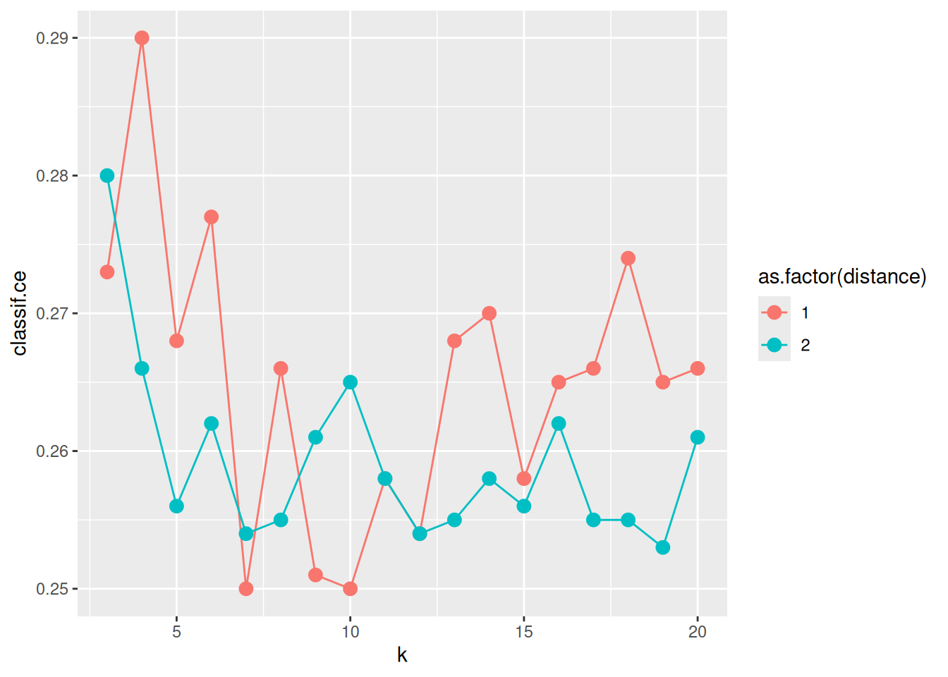

On average, the Euclidean distance (distance = 2) seems to work better. However, there is much randomness introduced by the resampling instance. So you, the reader, may see a different result, when you run the experiment yourself and set a different random seed. For k, we find that values between 7 and 13 perform well.

Random Search and Transformation

Let’s have a look at a larger search space. For example, we could tune all available parameters and limit k to large values (50). We also now tune the distance param continuously from 1 to 3 as a double and tune distance kernel and whether we scale the features.

We may find two problems when doing so:

First, the resulting difference in performance between k = 3 and k = 4 is probably larger than the difference between k = 49 and k = 50. While 4 is 33% larger than 3, 50 is only 2 percent larger than 49. To account for this we will use a transformation function for k and optimize in log-space. We define the range for k from log(3) to log(50) and exponentiate in the transformation. Now, as k has become a double instead of an int (in the search space, before transformation), we round it in the extra_trafo.

search_space_large = ps(
  k = p_dbl(log(3), log(50)),
  distance = p_dbl(1, 3),
  kernel = p_fct(c("rectangular", "gaussian", "rank", "optimal")),
  scale = p_lgl(),
  .extra_trafo = function(x, param_set) {
    x$k = round(exp(x$k))
    x
  }
)

The second problem is that grid search may (and often will) take a long time. For instance, trying out three different values for k, distance, kernel, and the two values for scale will take 54 evaluations. Because of this, we use a different search algorithm, namely the Random Search. We need to specify in the tuning instance a termination criterion. The criterion tells the search algorithm when to stop. Here, we will terminate after 36 evaluations:

tuner_random = tnr("random_search", batch_size = 36)

instance_random = TuningInstanceSingleCrit$new(
  task = task,
  learner = knn,
  resampling = cv10,
  measure = msr("classif.ce"),
  terminator = trm("evals", n_evals = 36),
  search_space = search_space_large
)

tuner_random$optimize(instance_random)

          k distance   kernel scale learner_param_vals  x_domain classif.ce
1: 1.683743 1.985146 gaussian  TRUE          <list[4]> <list[4]>      0.254

Like before, we can review the Archive. It includes the points before and after the transformation. The archive includes a column for each parameter the Tuner sampled on the search space (values before the transformation) and additional columns with prefix x_domain_* that refer to the parameters used by the learner (values after the transformation):

as.data.table(instance_random$archive)

Let’s now investigate the performance by parameters. This is especially easy using visualization:

ggplot(as.data.table(instance_random$archive),
  aes(x = x_domain_k, y = classif.ce, color = x_domain_scale)) +
  geom_point(size = 3) + geom_line()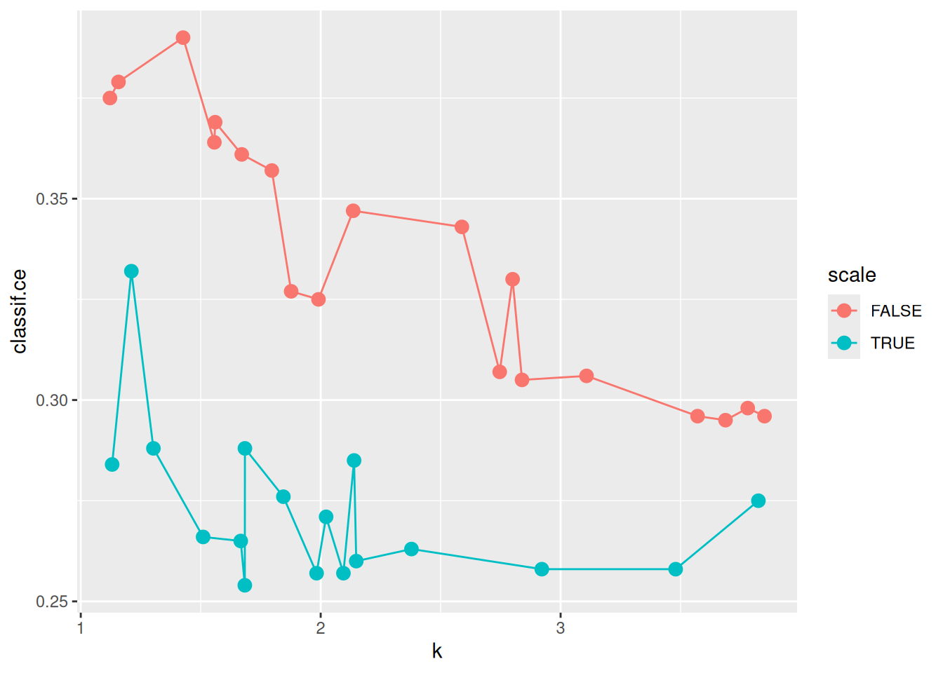

The previous plot suggests that scale has a strong influence on performance. For the kernel, there does not seem to be a strong influence:

ggplot(as.data.table(instance_random$archive),
  aes(x = x_domain_k, y = classif.ce, color = x_domain_kernel)) +
  geom_point(size = 3) + geom_line()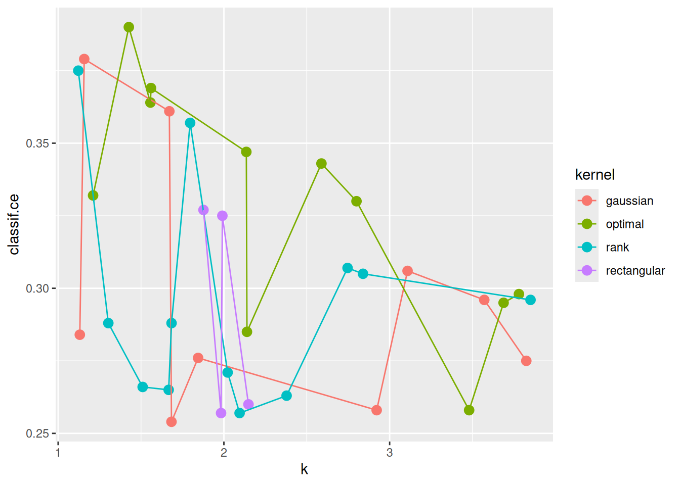

Nested Resampling

Having determined tuned configurations that seem to work well, we want to find out which performance we can expect from them. However, this may require more than this naive approach:

instance_random$result_y

classif.ce 
     0.254

instance_grid$result_y

classif.ce 
      0.25

The problem associated with evaluating tuned models is overtuning. The more we search, the more optimistically biased the associated performance metrics from tuning become.

There is a solution to this problem, namely Nested Resampling.

The mlr3tuning package provides an AutoTuner that acts like our tuning method but is actually a Learner. The $train() method facilitates tuning of hyperparameters on the training data, using a resampling strategy (below we use 5-fold cross-validation). Then, we actually train a model with optimal hyperparameters on the whole training data.

The AutoTuner finds the best parameters and uses them for training:

at_grid = AutoTuner$new(
  learner = knn,
  resampling = rsmp("cv", folds = 5), # we can NOT use fixed resampling here
  measure = msr("classif.ce"),
  terminator = trm("none"),
  tuner = tnr("grid_search", resolution = 18),
  search_space = search_space
)

The AutoTuner behaves just like a regular Learner. It can be used to combine the steps of hyperparameter tuning and model fitting but is especially useful for resampling and fair comparison of performance through benchmarking:

rr = resample(task, at_grid, cv10, store_models = TRUE)

We check the inner tuning results for stable hyperparameters. This means that the selected hyperparameters should not vary too much. We might observe unstable models in this example because the small data set and the low number of resampling iterations might introduce too much randomness. Usually, we aim for the selection of stable hyperparameters for all outer training sets.

extract_inner_tuning_results(rr)

    iteration  k distance classif.ce       task_id         learner_id resampling_id
 1:         1  7        1  0.2588889 german_credit classif.kknn.tuned            cv
 2:         2  5        2  0.2377778 german_credit classif.kknn.tuned            cv
 3:         3 10        2  0.2500000 german_credit classif.kknn.tuned            cv
 4:         4  9        2  0.2488889 german_credit classif.kknn.tuned            cv
 5:         5  7        2  0.2477778 german_credit classif.kknn.tuned            cv
 6:         6  8        2  0.2411111 german_credit classif.kknn.tuned            cv
 7:         7  8        2  0.2688889 german_credit classif.kknn.tuned            cv
 8:         8  7        2  0.2477778 german_credit classif.kknn.tuned            cv
 9:         9  7        2  0.2655556 german_credit classif.kknn.tuned            cv
10:        10  7        2  0.2455556 german_credit classif.kknn.tuned            cv

Next, we want to compare the predictive performances estimated on the outer resampling to the inner resampling (extract_inner_tuning_results(rr)). Significantly lower predictive performances on the outer resampling indicate that the models with the optimized hyperparameters overfit the data.

rr$score()

The archives of the AutoTuners allows us to inspect all evaluated hyperparameters configurations with the associated predictive performances.

extract_inner_tuning_archives(rr)

We aggregate the performances of all resampling iterations:

rr$aggregate()

classif.ce 
     0.255

Essentially, this is the performance of a “knn with optimal hyperparameters found by grid search”. Note that at_grid is not changed since resample() creates a clone for each resampling iteration.

The trained AutoTuner objects can be accessed by using

rr$learners[[1]]

<AutoTuner:classif.kknn.tuned>
* Model: list
* Search Space:
<ParamSet>
         id    class lower upper nlevels        default value
1:        k ParamInt     3    20      18 <NoDefault[3]>      
2: distance ParamInt     1     2       2 <NoDefault[3]>      
* Packages: mlr3, mlr3tuning, mlr3learners, kknn
* Predict Type: prob
* Feature Types: logical, integer, numeric, factor, ordered
* Properties: multiclass, twoclass

rr$learners[[1]]$tuning_result

   k distance learner_param_vals  x_domain classif.ce
1: 7        1          <list[3]> <list[2]>  0.2588889

Appendix

Example: Tuning With A Larger Budget

It is always interesting to look at what could have been. The following dataset contains an optimization run result with 3600 evaluations – more than above by a factor of 100:

The scale effect is just as visible as before with fewer data:

ggplot(perfdata, aes(x = x_domain_k, y = classif.ce, color = scale)) +
  geom_point(size = 2, alpha = 0.3)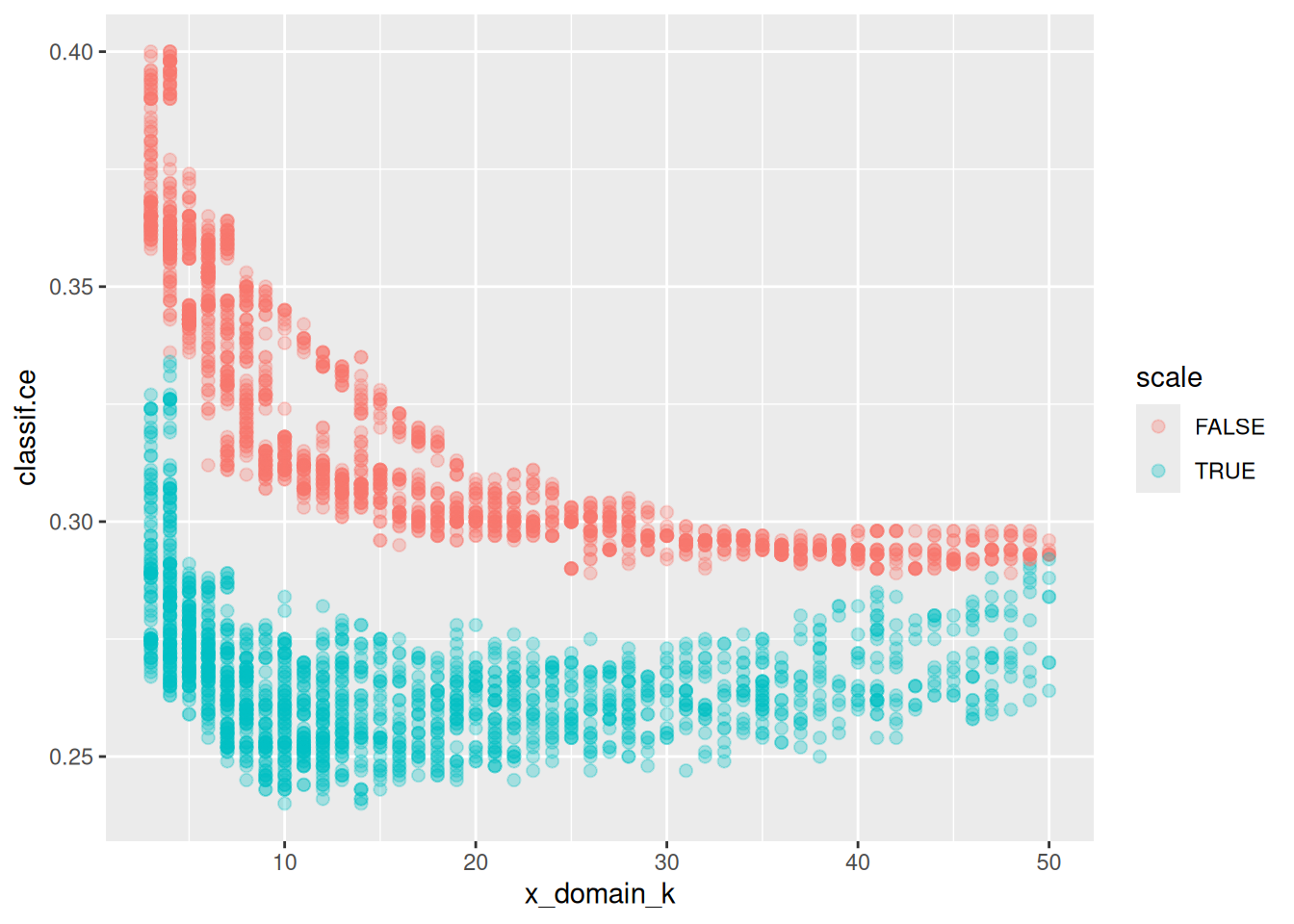

Now, there seems to be a visible pattern by kernel as well:

ggplot(perfdata, aes(x = x_domain_k, y = classif.ce, color = kernel)) +
  geom_point(size = 2, alpha = 0.3)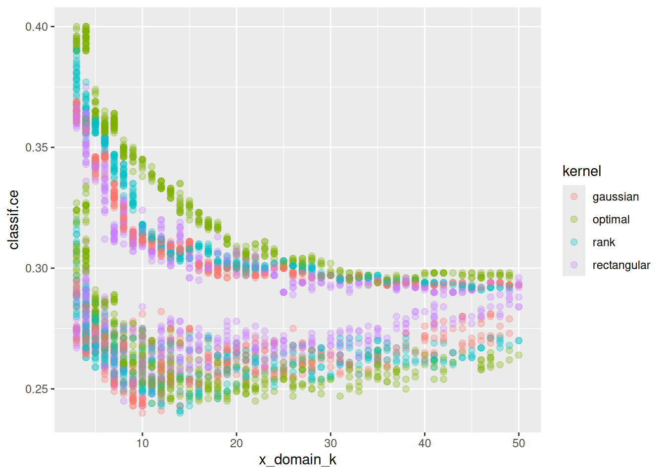

In fact, if we zoom in to (5, 40) $\times$ (0.23, 0.28) and do decrease smoothing we see that different kernels have their optimum at different values of k:

ggplot(perfdata, aes(x = x_domain_k, y = classif.ce, color = kernel,
  group = interaction(kernel, scale))) +
  geom_point(size = 2, alpha = 0.3) + geom_smooth() +
  xlim(5, 40) + ylim(0.23, 0.28)

`geom_smooth()` using method = 'loess' and formula = 'y ~ x'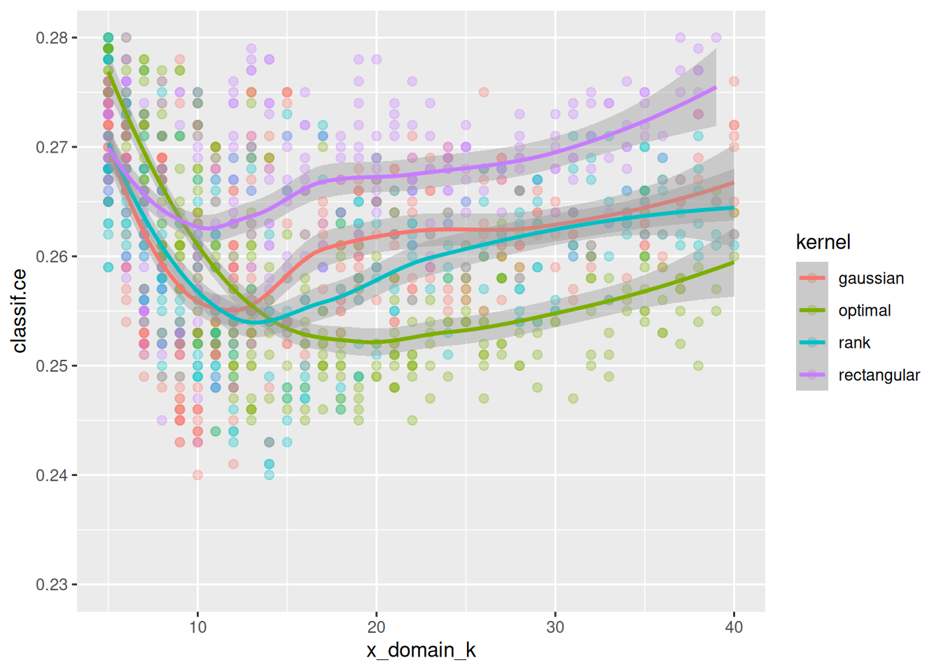

What about the distance parameter? If we select all results with k between 10 and 20 and plot distance and kernel we see an approximate relationship:

ggplot(perfdata[x_domain_k > 10 & x_domain_k < 20 & scale == TRUE],
  aes(x = distance, y = classif.ce, color = kernel)) +
  geom_point(size = 2) + geom_smooth()

`geom_smooth()` using method = 'loess' and formula = 'y ~ x'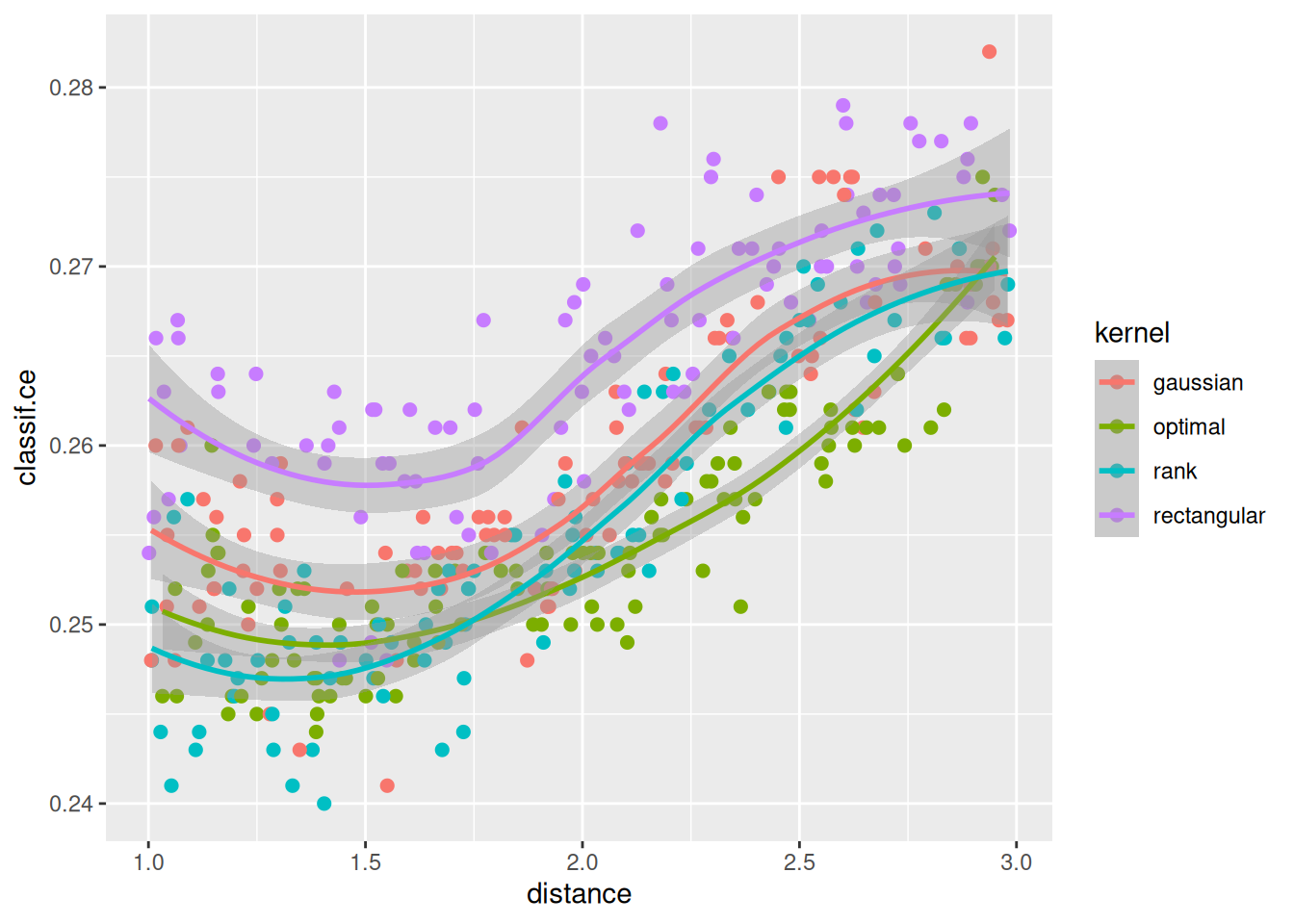

In sum our observations are: The scale parameter is very influential, and scaling is beneficial. The distance type seems to be the least influential. There seems to be an interaction between ‘k’ and ‘kernel’.