House Prices in King County

The use-case illustrated below touches on the following concepts:

• Data preprocessing
• Task
• Fitting a learner
• Resampling
• Tuning

The relevant sections in the mlr3book are linked to for the reader’s convenience.

This use case shows how to model housing price data in King County. Following features are illustrated:

• Summarizing the data set
• Converting data to treat it as a numeric feature/factor
• Generating new variables
• Splitting data into train and test data sets
• Computing a first model (decision tree)
• Building many trees (random forest)
• Visualizing price data across different region
• Optimizing the baseline by implementing a tuner
• Engineering features
• Creating a sparser model

We load the mlr3verse package which pulls in the most important packages for this example.

library(mlr3verse)

Loading required package: mlr3

We initialize the random number generator with a fixed seed for reproducibility, and decrease the verbosity of the logger to keep the output clearly represented.

set.seed(7832)
lgr::get_logger("mlr3")$set_threshold("warn")
lgr::get_logger("bbotk")$set_threshold("warn")

House Price Prediction in King County

We use the kc_housing dataset contained in the package mlr3data in order to provide a use-case for the application of mlr3 on real-world data.

data("kc_housing", package = "mlr3data")

Exploratory Data Analysis

In order to get a quick impression of our data, we perform some initial Exploratory Data Analysis. This helps us to get a first impression of our data and might help us arrive at additional features that can help with the prediction of the house prices.

We can get a quick overview using R’s summary function:

summary(kc_housing)

      date                           price            bedrooms        bathrooms      sqft_living       sqft_lot      
 Min.   :2014-05-02 00:00:00.0   Min.   :  75000   Min.   : 0.000   Min.   :0.000   Min.   :  290   Min.   :    520  
 1st Qu.:2014-07-22 00:00:00.0   1st Qu.: 321950   1st Qu.: 3.000   1st Qu.:1.750   1st Qu.: 1427   1st Qu.:   5040  
 Median :2014-10-16 00:00:00.0   Median : 450000   Median : 3.000   Median :2.250   Median : 1910   Median :   7618  
 Mean   :2014-10-29 03:58:09.9   Mean   : 540088   Mean   : 3.371   Mean   :2.115   Mean   : 2080   Mean   :  15107  
 3rd Qu.:2015-02-17 00:00:00.0   3rd Qu.: 645000   3rd Qu.: 4.000   3rd Qu.:2.500   3rd Qu.: 2550   3rd Qu.:  10688  
 Max.   :2015-05-27 00:00:00.0   Max.   :7700000   Max.   :33.000   Max.   :8.000   Max.   :13540   Max.   :1651359  
                                                                                                                     
     floors      waterfront           view          condition         grade          sqft_above   sqft_basement   
 Min.   :1.000   Mode :logical   Min.   :0.0000   Min.   :1.000   Min.   : 1.000   Min.   : 290   Min.   :  10.0  
 1st Qu.:1.000   FALSE:21450     1st Qu.:0.0000   1st Qu.:3.000   1st Qu.: 7.000   1st Qu.:1190   1st Qu.: 450.0  
 Median :1.500   TRUE :163       Median :0.0000   Median :3.000   Median : 7.000   Median :1560   Median : 700.0  
 Mean   :1.494                   Mean   :0.2343   Mean   :3.409   Mean   : 7.657   Mean   :1788   Mean   : 742.4  
 3rd Qu.:2.000                   3rd Qu.:0.0000   3rd Qu.:4.000   3rd Qu.: 8.000   3rd Qu.:2210   3rd Qu.: 980.0  
 Max.   :3.500                   Max.   :4.0000   Max.   :5.000   Max.   :13.000   Max.   :9410   Max.   :4820.0  
                                                                                                  NA's   :13126   
    yr_built     yr_renovated      zipcode           lat             long        sqft_living15    sqft_lot15    
 Min.   :1900   Min.   :1934    Min.   :98001   Min.   :47.16   Min.   :-122.5   Min.   : 399   Min.   :   651  
 1st Qu.:1951   1st Qu.:1987    1st Qu.:98033   1st Qu.:47.47   1st Qu.:-122.3   1st Qu.:1490   1st Qu.:  5100  
 Median :1975   Median :2000    Median :98065   Median :47.57   Median :-122.2   Median :1840   Median :  7620  
 Mean   :1971   Mean   :1996    Mean   :98078   Mean   :47.56   Mean   :-122.2   Mean   :1987   Mean   : 12768  
 3rd Qu.:1997   3rd Qu.:2007    3rd Qu.:98118   3rd Qu.:47.68   3rd Qu.:-122.1   3rd Qu.:2360   3rd Qu.: 10083  
 Max.   :2015   Max.   :2015    Max.   :98199   Max.   :47.78   Max.   :-121.3   Max.   :6210   Max.   :871200  
                NA's   :20699                                                                                   

dim(kc_housing)

[1] 21613    20

Our dataset has 21613 observations and 20 columns. The variable we want to predict is price. In addition to the price column, we have several other columns:

• id: A unique identifier for every house.

• date: A date column, indicating when the house was sold. This column is currently not encoded as a date and requires some preprocessing.

• zipcode: A column indicating the ZIP code. This is a categorical variable with many factor levels.

• long, lat The longitude and latitude of the house

• ... several other numeric columns providing information about the house, such as number of rooms, square feet etc.

Before we continue with the analysis, we preprocess some features so that they are stored in the correct format.

First we convert the date column to numeric. To do so, we convert the date to the POSIXct date/time class with the anytime package. Next, use difftime() to convert to days since the first day recorded in the data set:

library(anytime)
dates = anytime(kc_housing$date)
kc_housing$date = as.numeric(difftime(dates, min(dates), units = "days"))

Afterwards, we convert the zip code to a factor:

kc_housing$zipcode = as.factor(kc_housing$zipcode)

And add a new column renovated indicating whether a house was renovated at some point.

kc_housing$renovated = as.numeric(!is.na(kc_housing$yr_renovated))
kc_housing$has_basement = as.numeric(!is.na(kc_housing$sqft_basement))

We drop the id column which provides no information about the house prices:

kc_housing$id = NULL

Additionally, we convert the price from Dollar to units of 1000 Dollar to improve readability.

kc_housing$price = kc_housing$price / 1000

Additionally, for now we simply drop the columns that have missing values, as some of our learners can not deal with them. A better option to deal with missing values would be imputation, i.e. replacing missing values with valid ones. We will deal with this in a separate article.

kc_housing$yr_renovated = NULL
kc_housing$sqft_basement = NULL

We can now plot the density of the price to get a first impression on its distribution.

library(ggplot2)
ggplot(kc_housing, aes(x = price)) + geom_density()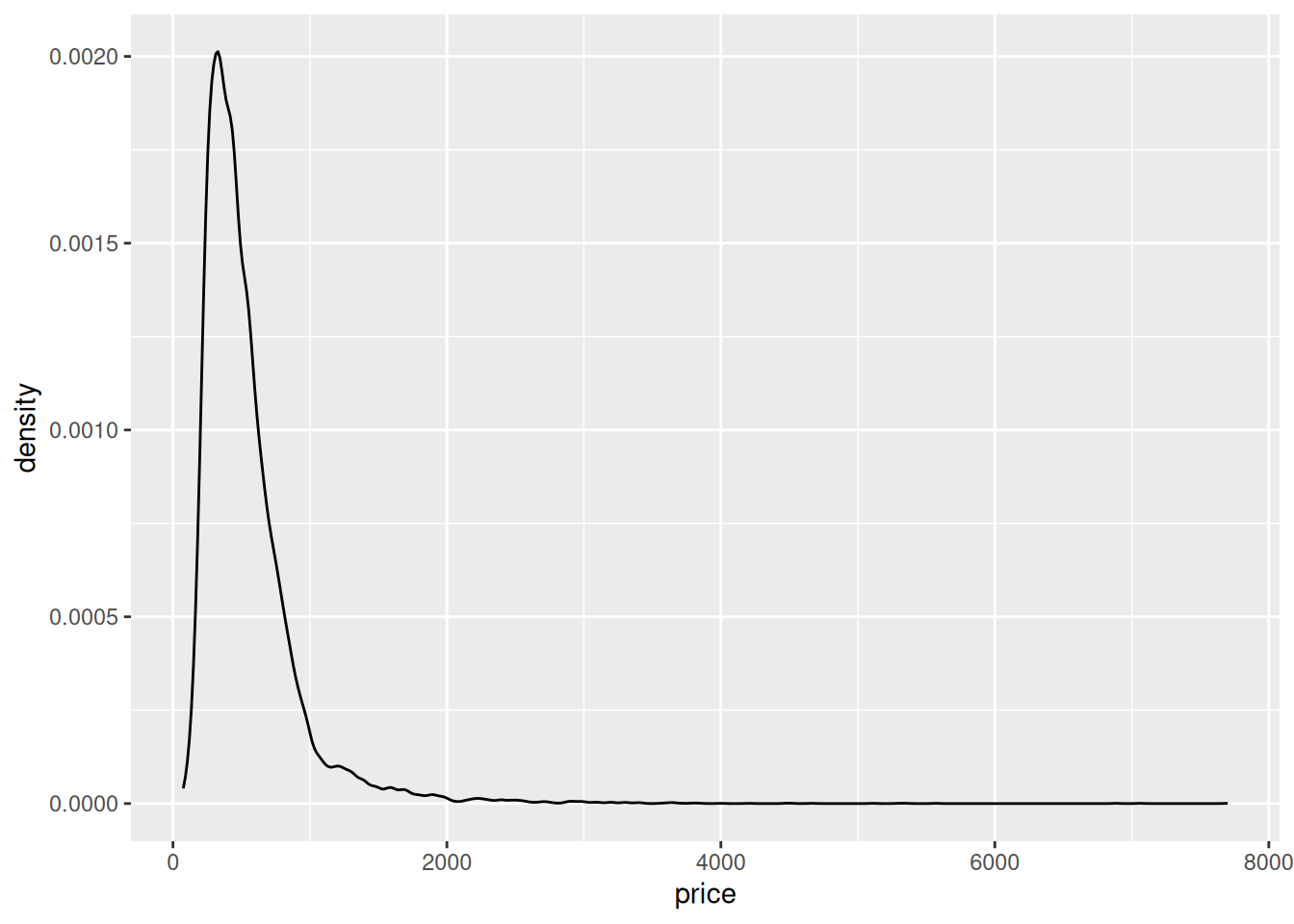

We can see that the prices for most houses lie between 75.000 and 1.5 million dollars. There are few extreme values of up to 7.7 million dollars.

Feature engineering often allows us to incorporate additional knowledge about the data and underlying processes. This can often greatly enhance predictive performance. A simple example: A house which has yr_renovated == 0 means that is has not been renovated yet. Additionally, we want to drop features which should not have any influence (id column).

After those initial manipulations, we load all required packages and create a TaskRegr containing our data.

tsk = as_task_regr(kc_housing, target = "price")

We can inspect associations between variables using mlr3viz’s autoplot function in order to get some good first impressions for our data. Note, that this does in no way prevent us from using other powerful plot functions of our choice on the original data.

Distribution of the price:

The outcome we want to predict is the price variable. The autoplot function provides a good first glimpse on our data. As the resulting object is a ggplot2 object, we can use faceting and other functions from ggplot2 in order to enhance plots.

autoplot(tsk) + facet_wrap(~renovated)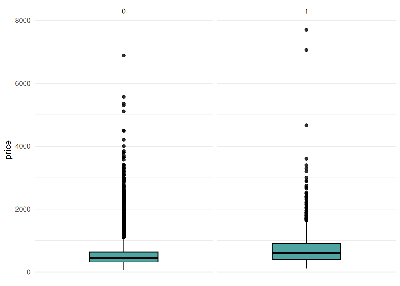

We can observe that renovated flats seem to achieve higher sales values, and this might thus be a relevant feature.

Additionally, we can for example look at the condition of the house. Again, we clearly can see that the price rises with increasing condition.

autoplot(tsk) + facet_wrap(~condition)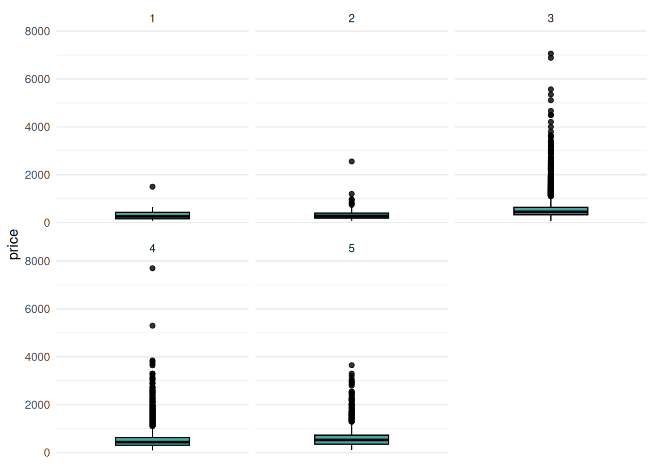

Association between variables

In addition to the association with the target variable, the association between the features can also lead to interesting insights. We investigate using variables associated with the quality and size of the house. Note that we use $clone() and $select() to clone the task and select only a subset of the features for the autoplot function, as autoplot per default uses all features. The task is cloned before we select features in order to keep the original task intact.

# Variables associated with quality
autoplot(tsk$clone()$select(tsk$feature_names[c(3, 17)]), type = "pairs")

Registered S3 method overwritten by 'GGally':
  method from   
  +.gg   ggplot2

`stat_bin()` using `bins = 30`. Pick better value with `binwidth`.
`stat_bin()` using `bins = 30`. Pick better value with `binw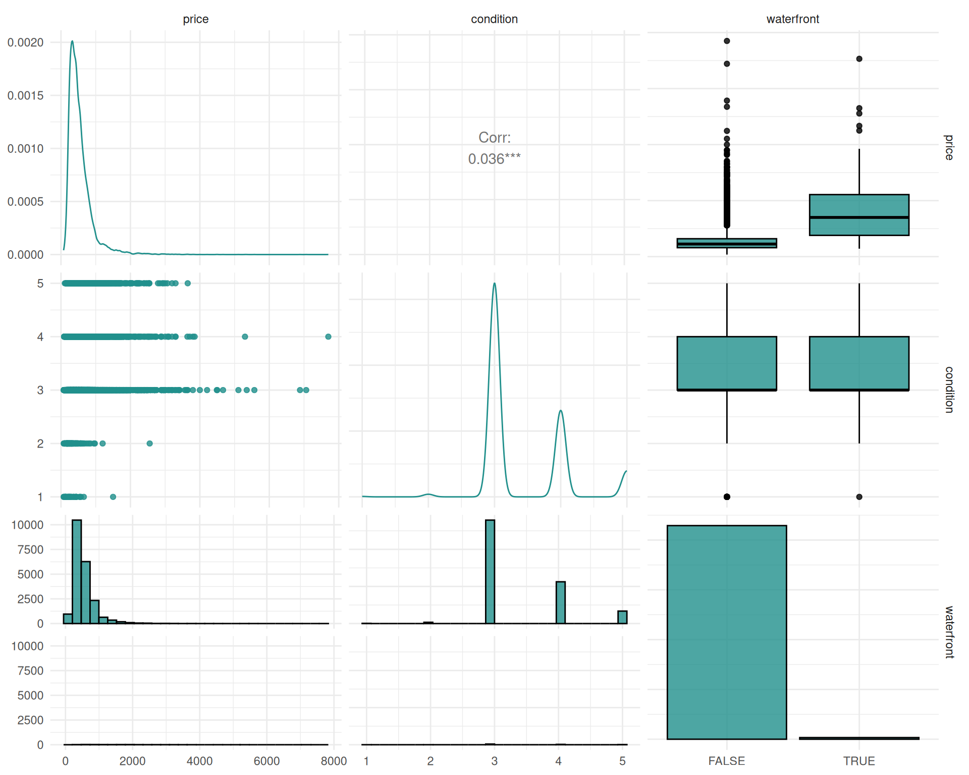idth`.

autoplot(tsk$clone()$select(tsk$feature_names[c(9:12)]), type = "pairs")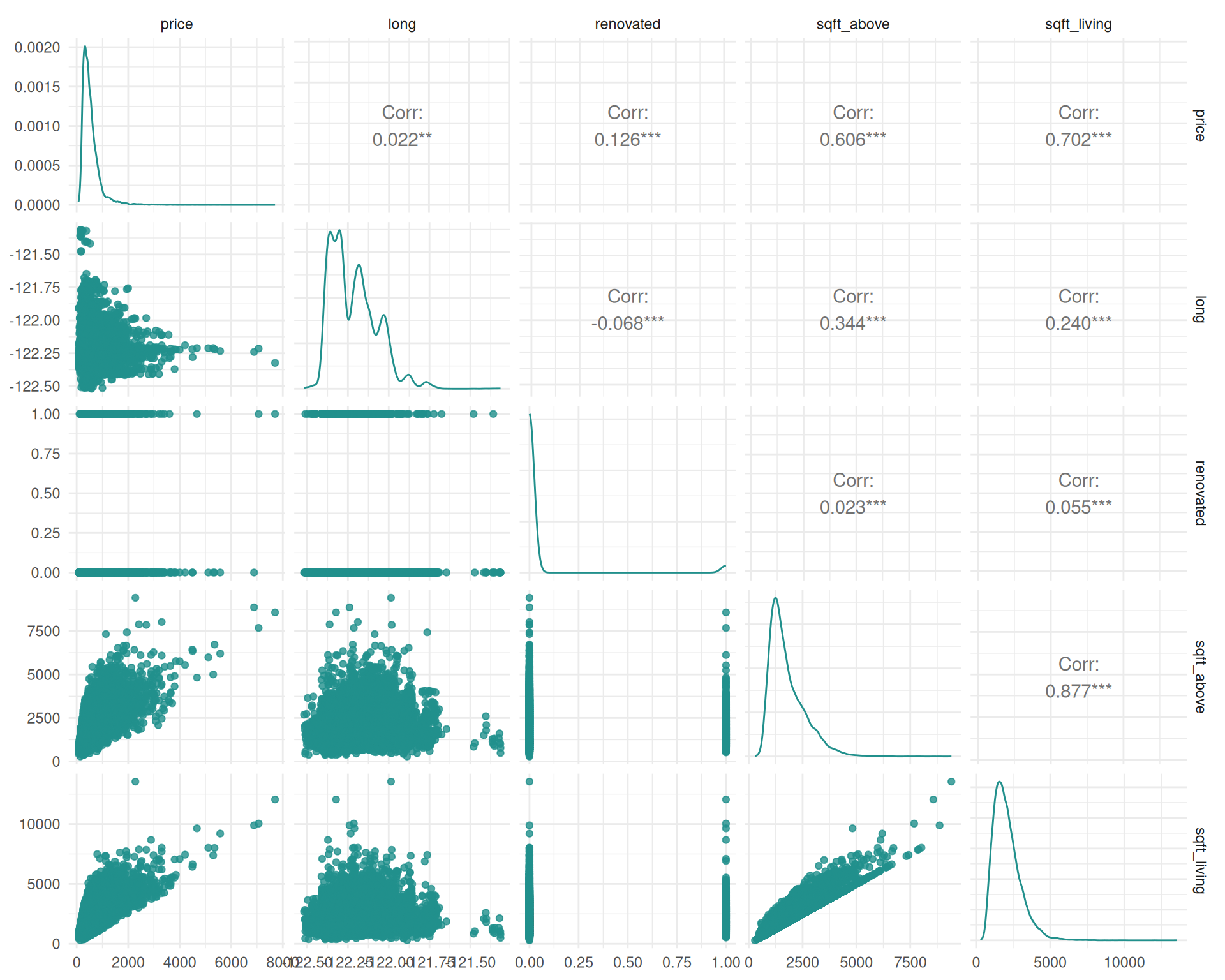

Splitting into train and test data

In mlr3, we do not create train and test data sets, but instead keep only a vector of train and test indices.

train.idx = sample(seq_len(tsk$nrow), 0.7 * tsk$nrow)
test.idx = setdiff(seq_len(tsk$nrow), train.idx)

We can do the same for our task:

task_train = tsk$clone()$filter(train.idx)
task_test = tsk$clone()$filter(test.idx)

A first model: Decision Tree

Decision trees cannot only be used as a powerful tool for predictive models but also for exploratory data analysis. In order to fit a decision tree, we first get the regr.rpart learner from the mlr_learners dictionary by using the sugar function lrn.

For now, we leave out the zipcode variable, as we also have the latitude and longitude of each house. Again, we use $clone(), so we do not change the original task.

tsk_nozip = task_train$clone()$select(setdiff(tsk$feature_names, "zipcode"))

# Get the learner
lrn = lrn("regr.rpart")

# And train on the task
lrn$train(tsk_nozip, row_ids = train.idx)

plot(lrn$model)
text(lrn$model)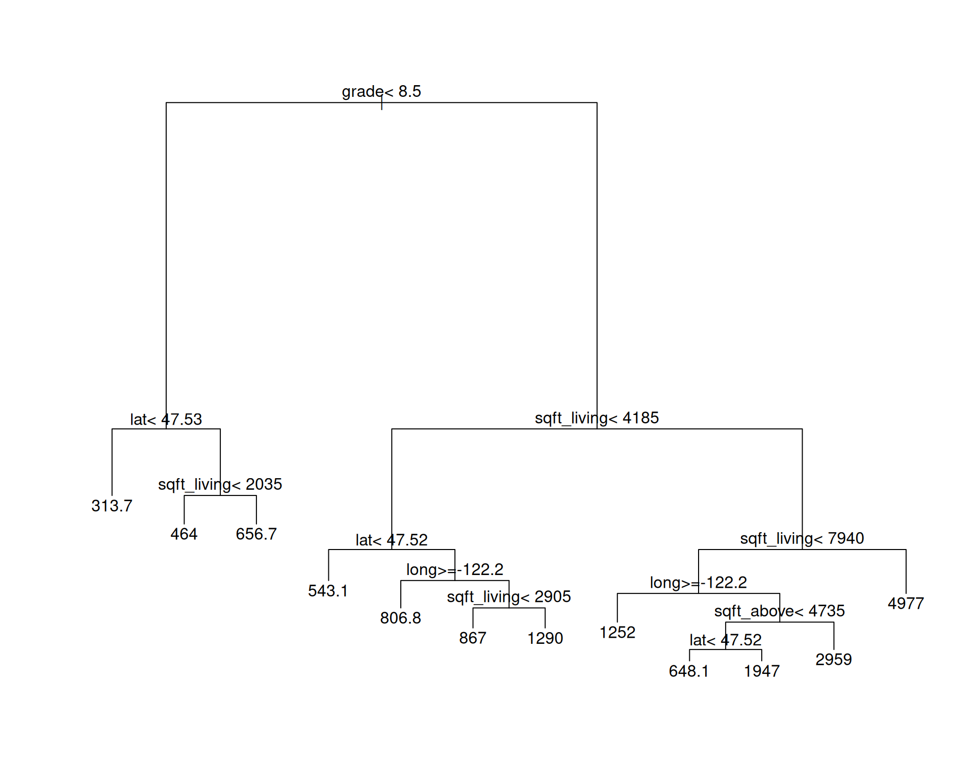

The learned tree relies on several variables in order to distinguish between cheaper and pricier houses. The features we split along are grade, sqft_living, but also some features related to the area (longitude and latitude). We can visualize the price across different regions in order to get more info:

# Load the ggmap package in order to visualize on a map
library(ggmap)

# And create a quick plot for the price
qmplot(long, lat, maptype = "watercolor", color = log(price),
  data = kc_housing[train.idx[1:3000], ]) +
  scale_colour_viridis_c()

# And the zipcode
qmplot(long, lat, maptype = "watercolor", color = zipcode,
  data = kc_housing[train.idx[1:3000], ]) + guides(color = FALSE)

Warning: The `<scale>` argument of `guides()` cannot be `FALSE`. Use "none" instead as of ggplot2 3.3.4.

We can see that the price is clearly associated with the zipcode when comparing then two plots. As a result, we might want to indeed use the zipcode column in our future endeavors.

A first baseline: Decision Tree

After getting an initial idea for our data, we might want to construct a first baseline, in order to see what a simple model already can achieve.

We use resample() with 3-fold cross-validation on our training data in order to get a reliable estimate of the algorithm’s performance on future data. Before we start with defining and training learners, we create a Resampling in order to make sure that we always compare on exactly the same data.

cv3 = rsmp("cv", folds = 3)

For the cross-validation we only use the training data by cloning the task and selecting only observations from the training set.

lrn_rpart = lrn("regr.rpart")
res = resample(task = task_train, lrn_rpart, cv3)
res$score(msr("regr.rmse"))

      task_id learner_id resampling_id iteration regr.rmse
1: kc_housing regr.rpart            cv         1  205.7541
2: kc_housing regr.rpart            cv         2  205.6597
3: kc_housing regr.rpart            cv         3  213.3846
Hidden columns: task, learner, resampling, prediction

sprintf("RMSE of the simple rpart: %s", round(sqrt(res$aggregate()), 2))

[1] "RMSE of the simple rpart: 208.3"

Many Trees: Random Forest

We might be able to improve upon the RMSE using more powerful learners. We first load the mlr3learners package, which contains the ranger learner (a package which implements the “Random Forest” algorithm).

library(mlr3learners)
lrn_ranger = lrn("regr.ranger", num.trees = 15L)
res = resample(task = task_train, lrn_ranger, cv3)
res$score(msr("regr.rmse"))

      task_id  learner_id resampling_id iteration regr.rmse
1: kc_housing regr.ranger            cv         1  142.2424
2: kc_housing regr.ranger            cv         2  161.6867
3: kc_housing regr.ranger            cv         3  138.2549
Hidden columns: task, learner, resampling, prediction

sprintf("RMSE of the simple ranger: %s", round(sqrt(res$aggregate()), 2))

[1] "RMSE of the simple ranger: 147.75"

Often tuning RandomForest methods does not increase predictive performances substantially. If time permits, it can nonetheless lead to improvements and should thus be performed. In this case, we resort to tune a different kind of model: Gradient Boosted Decision Trees from the package xgboost.

A better baseline: AutoTuner

Tuning can often further improve the performance. In this case, we tune the xgboost learner in order to see whether this can improve performance. For the AutoTuner we have to specify a Termination Criterion (how long the tuning should run) a Tuner (which tuning method to use) and a ParamSet (which space we might want to search through). For now, we do not use the zipcode column, as xgboost cannot naturally deal with categorical features. The AutoTuner automatically performs nested cross-validation.

lrn_xgb = lrn("regr.xgboost")

# Define the search space
search_space = ps(
  eta = p_dbl(lower = 0.2, upper = .4),
  min_child_weight = p_dbl(lower = 1, upper = 20),
  subsample = p_dbl(lower = .7, upper = .8),
  colsample_bytree = p_dbl(lower = .9, upper = 1),
  colsample_bylevel = p_dbl(lower = .5, upper = .7),
  nrounds = p_int(lower = 1L, upper = 25))

at = auto_tuner(
  tuner = tnr("random_search", batch_size = 40),
  learner = lrn_xgb,
  resampling = rsmp("holdout"),
  measure = msr("regr.rmse"),
  search_space = search_space,
  term_evals = 10)

# And resample the AutoTuner
res = resample(tsk_nozip, at, cv3, store_models = TRUE)

res$score(msr("regr.rmse"))

      task_id         learner_id resampling_id iteration regr.rmse
1: kc_housing regr.xgboost.tuned            cv         1  147.0554
2: kc_housing regr.xgboost.tuned            cv         2  136.4282
3: kc_housing regr.xgboost.tuned            cv         3  132.4484
Hidden columns: task, learner, resampling, prediction

sprintf("RMSE of the tuned xgboost: %s", round(sqrt(res$aggregate()), 2))

[1] "RMSE of the tuned xgboost: 138.78"

We can obtain the resulting parameters in the respective splits by accessing the ResampleResult.

sapply(res$learners, function(x) x$learner$param_set$values)[-2, ]

                   [,1]      [,2]      [,3]     
nrounds            25        23        24       
verbose            0         0         0        
early_stopping_set "none"    "none"    "none"   
eta                0.220869  0.3809271 0.2115116
min_child_weight   1.885109  7.472919  1.910491 
subsample          0.7542127 0.7884631 0.7000357
colsample_bytree   0.9032271 0.9675298 0.9120812
colsample_bylevel  0.5259713 0.6817893 0.630818 

NOTE: To keep runtime low, we only tune parts of the hyperparameter space of xgboost in this example. Additionally, we only allow for \(10\) random search iterations, which is usually too little for real-world applications. Nonetheless, we are able to obtain an improved performance when comparing to the ranger model.

In order to further improve our results we have several options:

• Find or engineer better features
• Remove Features to avoid overfitting
• Obtain additional data (often prohibitive)
• Try more models
• Improve the tuning
  • Increase the tuning budget
  • Enlarge the tuning search space
  • Use a more efficient tuning algorithm
• Stacking and Ensembles

Below we will investigate some of those possibilities and investigate whether this improves performance.

Advanced: Engineering Features: Mutating ZIP-Codes

In order to better cluster the zip codes, we compute a new feature: med_price: It computes the median price in each zip-code. This might help our model to improve the prediction. This is equivalent to impact encoding more information:

We can equip a learner with impact encoding using mlr3pipelines. More information on mlr3pipelines can be obtained from other posts.

lrn_impact = po("encodeimpact", affect_columns = selector_name("zipcode")) %>>% lrn("regr.ranger")

Again, we run resample() and compute the RMSE.

res = resample(task = task_train, lrn_impact, cv3)

res$score(msr("regr.rmse"))

      task_id               learner_id resampling_id iteration regr.rmse
1: kc_housing encodeimpact.regr.ranger            cv         1  119.4597
2: kc_housing encodeimpact.regr.ranger            cv         2  146.3315
3: kc_housing encodeimpact.regr.ranger            cv         3  125.4193
Hidden columns: task, learner, resampling, prediction

sprintf("RMSE of ranger with med_price: %s", round(sqrt(res$aggregate()), 2))

[1] "RMSE of ranger with med_price: 130.91"

Advanced: Obtaining a sparser model

In many cases, we might want to have a sparse model. For this purpose we can use a mlr3filters::Filter implemented in mlr3filters. This can prevent our learner from overfitting make it easier for humans to interpret models as fewer variables influence the resulting prediction.

In this example, we use PipeOpFilter (via po("filter", ...)) to add a feature-filter before training the model. For a more in-depth insight, refer to the sections on mlr3pipelines and mlr3filters in the mlr3 book: Feature Selection and Pipelines.

filter = flt("mrmr")

The resulting RMSE is slightly higher, and at the same time we only use \(12\) features.

graph = po("filter", filter, param_vals = list(filter.nfeat = 12)) %>>% po("learner", lrn("regr.ranger"))
lrn_filter = as_learner(graph)
res = resample(task = task_train, lrn_filter, cv3)

res$score(msr("regr.rmse"))

      task_id       learner_id resampling_id iteration regr.rmse
1: kc_housing mrmr.regr.ranger            cv         1  152.6009
2: kc_housing mrmr.regr.ranger            cv         2  156.7883
3: kc_housing mrmr.regr.ranger            cv         3  149.0143
Hidden columns: task, learner, resampling, prediction

sprintf("RMSE of ranger with filtering: %s", round(sqrt(res$aggregate()), 2))

[1] "RMSE of ranger with filtering: 152.83"

Summary:

We have seen different ways to improve models with respect to our criteria by:

• Choosing a suitable algorithm
• Choosing good hyperparameters (tuning)
• Filtering features
• Engineering new features

A combination of all the above would most likely yield an even better model. This is left as an exercise to the reader.

The best model we found in this example is the ranger model with the added med_price feature. In a final step, we now want to assess the model’s quality on the held-out data we stored in our task_test. In order to do so, and to prevent data leakage, we can only add the median price from the training data.

library(data.table)

data = task_train$data(cols = c("price", "zipcode"))
data[, med_price := median(price), by = "zipcode"]
test_data = task_test$data(cols = "zipcode")
test = merge(test_data, unique(data[, .(zipcode, med_price)]), all.x = TRUE)
task_test$cbind(test)

Now we can use the augmented task_test to predict on new data.

lrn_ranger$train(task_train)
pred = lrn_ranger$predict(task_test)
pred$score(msr("regr.rmse"))

regr.rmse 
   145.01