library(mlr3verse)Loading required package: mlr3This tutorial assumes familiarity with the basics of mlr3pipelines. Consult the mlr3book if some aspects are not fully understandable. It deals with the problem of missing data.
The random forest implementation in the package ranger unfortunately does not support missing values. Therefore, it is required to impute missing features before passing the data to the learner.
We show how to use mlr3pipelines to augment the ranger learner with automatic imputation.
We load the mlr3verse package which pulls in the most important packages for this example.
library(mlr3verse)Loading required package: mlr3We initialize the random number generator with a fixed seed for reproducibility, and decrease the verbosity of the logger to keep the output clearly represented.
set.seed(7832)
lgr::get_logger("mlr3")$set_threshold("warn")First, we take an example task with missing values (diabetes) and create the ranger learner:
library(mlr3learners)

task = tsk("diabetes")
print(task)
── <TaskClassif> (128x9): Synthetic Diabetes ───────────────────────────────────────────────────────────────────────────
• Target: diabetes
• Properties: twoclass
• Features (8):
  • dbl (6): glucose, insulin, mass, pedigree, pressure, triceps
  • int (2): age, pregnant
• Target classes: pos (positive class, 35%), neg (65%)
learner = lrn("classif.ranger")
print(learner)
── <LearnerClassifRanger> (classif.ranger): Random Forest ──────────────────────────────────────────────────────────────
• Model: -
• Parameters: num.threads=1
• Packages: mlr3, mlr3learners, and ranger
• Predict Types: [response] and prob
• Feature Types: logical, integer, numeric, character, factor, and ordered
• Encapsulation: none (fallback: -)
• Properties: hotstart_backward, importance, missings, multiclass, oob_error, selected_features, twoclass, and weights
• Other settings: use_weights = 'use', predict_raw = 'FALSE'
We can now inspect the task for missing values. task$missings() returns the count of missing values for each variable.
task$missings()diabetes age glucose insulin mass pedigree pregnant pressure triceps
0 0 6 5 5 0 0 6 5 Additionally, we can see that the ranger learner can not handle missing values:
learner$properties[1] "hotstart_backward" "importance" "missings" "multiclass" "oob_error"
[6] "selected_features" "twoclass" "weights" For comparison, other learners, e.g. the rpart learner can handle missing values internally.
lrn("classif.rpart")$properties[1] "importance" "missings" "multiclass" "selected_features" "twoclass"
[6] "weights" Before we dive deeper, we quickly try to visualize two of the columns with missing values:
autoplot(task$clone()$select(c("insulin", "triceps")), type = "pairs")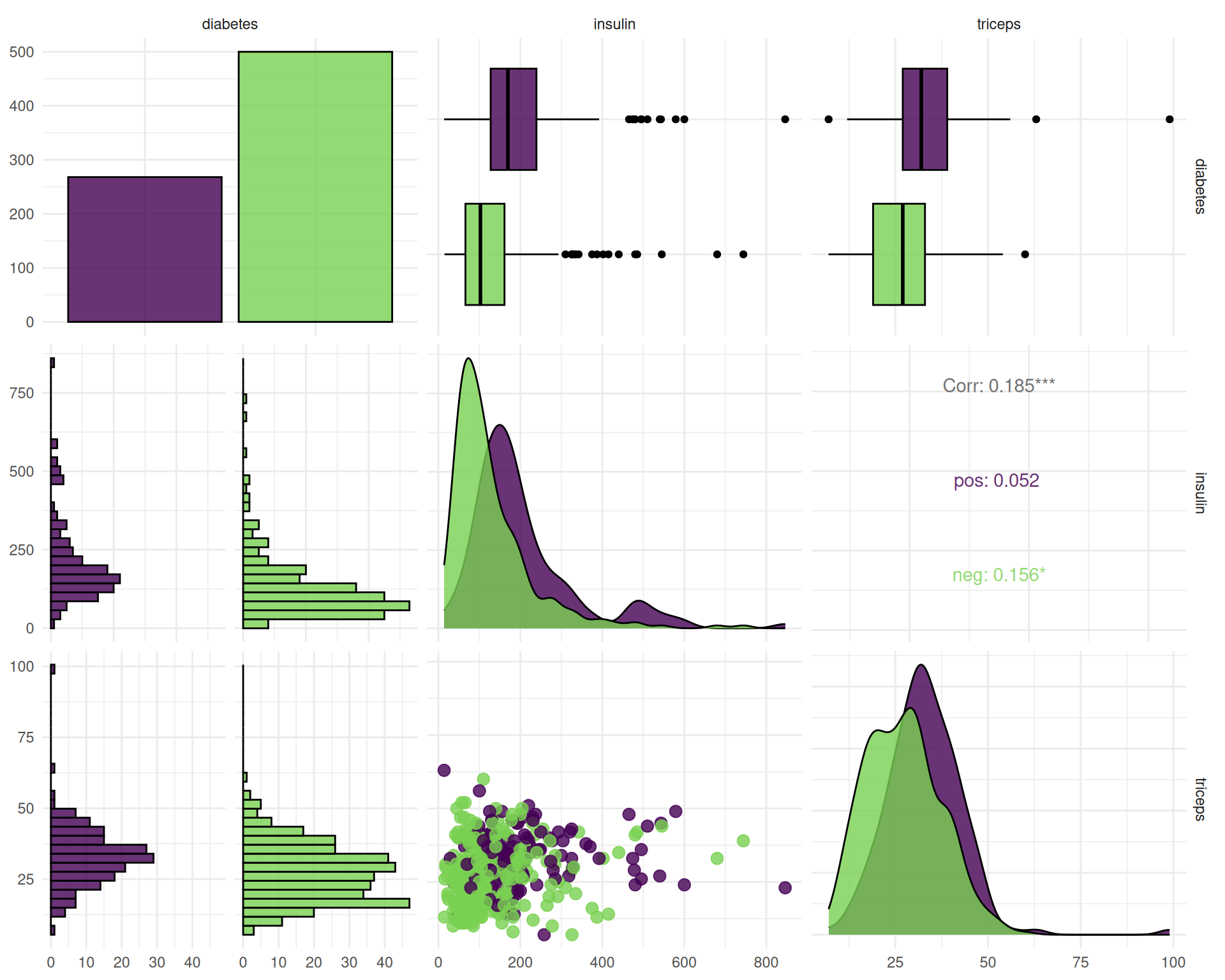
An overview over implemented PipeOps for imputation can be obtained like so:
mlr_pipeops$keys("^impute")[1] "imputeconstant" "imputehist" "imputelearner" "imputemean" "imputemedian" "imputemode"
[7] "imputeoor" "imputesample" mlr3pipelines contains several imputation methods. We focus on rather simple ones, and show how to impute missing values for factor features and numeric features respectively.
Since our task only has numeric features, we do not need to deal with imputing factor levels, and can instead concentrate on imputing numeric values:
We do this in a two-step process: * We create new indicator columns, that tells us whether the value of a feature is “missing” or “present”. We achieve this using the missind PipeOp.
imputehist PipeOp.We also have to make sure to apply the pipe operators in the correct order!
imp_missind = po("missind")
imp_num = po("imputehist", affect_columns = selector_type("numeric"))
In order to better understand we can look at the results of every PipeOp separately.
We can manually trigger the PipeOp to test the operator on our task:
task_ext = imp_missind$train(list(task))[[1]]
task_ext$data()
diabetes missing_glucose missing_insulin missing_mass missing_pressure missing_triceps
<fctr> <fctr> <fctr> <fctr> <fctr> <fctr>
1: pos missing present present present present
2: pos present present present missing present
3: neg present present present present missing
4: pos present missing present present present
5: neg present present missing present present
---
124: neg present present present present present
125: neg present present present present present
126: neg present present present present present
127: neg present present present missing present
128: neg present present present present presentFor imputehist, we can do the same:
task_ext = imp_num$train(list(task))[[1]]
task_ext$data()
diabetes age pedigree pregnant glucose insulin mass pressure triceps
<fctr> <int> <num> <int> <num> <num> <num> <num> <num>
1: pos 38 0.106 4 94.80615 15.0000 21.90000 84.00000 30.00000
2: pos 32 0.646 4 159.00000 84.0000 32.50000 94.63520 15.00000
3: neg 34 0.067 7 66.00000 62.0000 32.50000 89.00000 19.44956
4: pos 37 1.778 4 128.00000 158.3021 35.90000 58.00000 18.00000
5: neg 33 0.218 3 111.00000 206.0000 28.40266 79.00000 37.00000
---
124: neg 36 0.299 2 91.00000 82.0000 36.40000 86.00000 19.00000
125: neg 35 0.245 4 95.00000 69.0000 39.90000 102.00000 44.00000
126: neg 37 1.754 1 100.00000 51.0000 21.30000 74.00000 26.00000
127: neg 36 0.584 2 111.00000 210.0000 37.60000 62.16366 24.00000
128: neg 29 0.302 6 116.00000 66.0000 28.80000 63.00000 6.00000This time we obtain the imputed data set without missing values.
task_ext$missings()diabetes age pedigree pregnant glucose insulin mass pressure triceps
0 0 0 0 0 0 0 0 0 Now we have to put all PipeOps together in order to form a graph that handles imputation automatically.
We do this by creating a Graph that copies the data twice, processes each copy using the respective imputation method and afterwards unions the features. For this we need the following two PipeOps : * copy: Creates copies of the data. * featureunion Merges the two tasks together.
graph = po("copy", 2) %>>%
  gunion(list(imp_missind, imp_num)) %>>%
  po("featureunion")
as a last step we append the learner we planned on using:
graph = graph %>>% po(learner)We can now visualize the resulting graph:
graph$plot()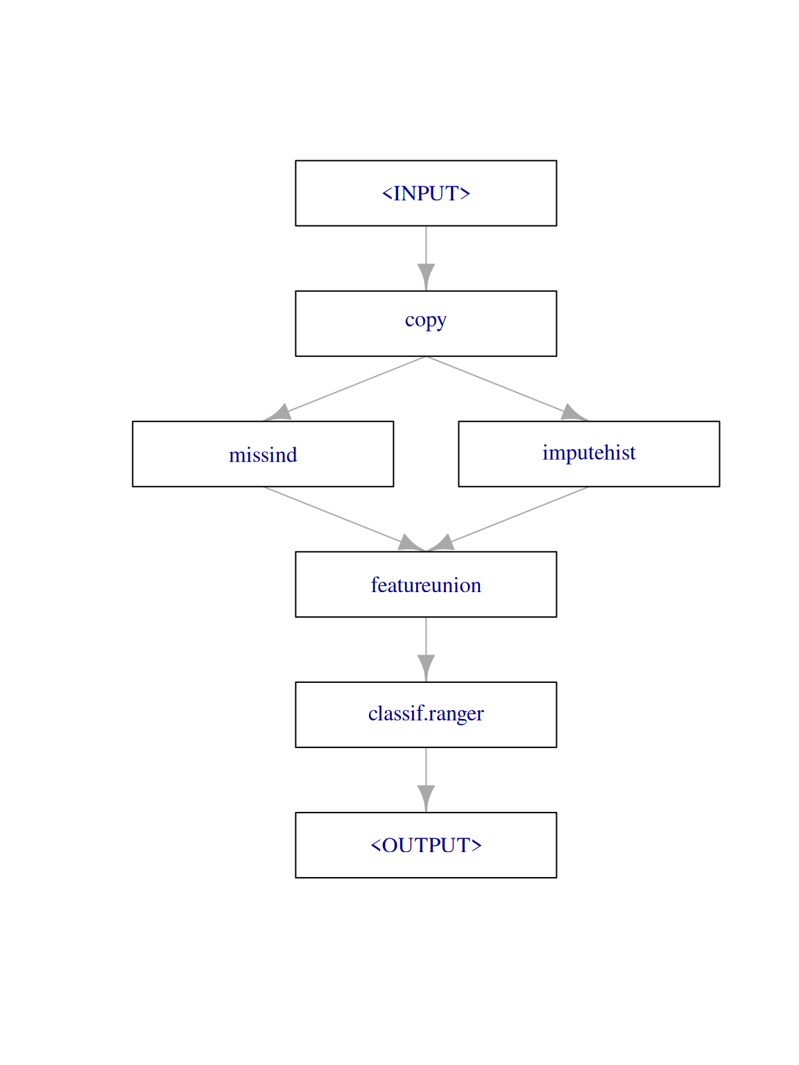
Correct imputation is especially important when applying imputation to held-out data during the predict step. If applied incorrectly, imputation could leak info from the test set, which potentially skews our performance estimates. mlr3pipelines takes this complexity away from the user and handles correct imputation internally.
By wrapping this graph into a GraphLearner, we can now train resample the full graph, here with a 3-fold cross validation:
graph_learner = as_learner(graph)
rr = resample(task, graph_learner, rsmp("cv", folds = 3))
rr$aggregate()
classif.ce
0.3589886 In some cases, we have missing values only in the data we want to predict on. In order to showcase this, we create a copy of the task with several more missing columns.
dt = task$data()
dt[1:10, "age"] = NA
dt[30:70, "pedigree"] = NA
task_2 = as_task_classif(dt, id = "diabetes2", target = "diabetes")
And now we learn on task, while trying to predict on task_2.
graph_learner$train(task)
graph_learner$predict(task_2)
── <PredictionClassif> for 128 observations: ───────────────────────────────────────────────────────────────────────────
 row_ids truth response
       1   pos      neg
       2   pos      pos
       3   neg      neg
     ---   ---      ---
     126   neg      neg
     127   neg      neg
128 neg negFor factor features, the process works analogously. Instead of using imputehist, we can for example use imputeoor. This will simply replace every NA in each factor variable with a new value missing.
A full graph might the look like this:
imp_missind = po("missind", affect_columns = NULL, which = "all")
imp_fct = po("imputeoor", affect_columns = selector_type("factor"))
graph = po("copy", 2) %>>%
  gunion(list(imp_missind, imp_num %>>% imp_fct)) %>>%
  po("featureunion")
Note that we specify the parameter affect_columns = NULL when initializing missind, because we also want indicator columns for our factor features. By default, affect_columns would be set to selector_invert(selector_type(c("factor", "ordered", "character"))). We also set the parameter which to "all" to add indicator columns for all features, regardless whether values were missing during training or not.
In order to test out our new graph, we again create a situation where our task has missing factor levels. As the (diabetes) task does not have any factor levels, we use the famous (boston_housing) task.
# task_bh_1 is the training data without missings
task_bh_1 = tsk("boston_housing")

# task_bh_2 is the prediction data with missings
dt = task_bh_1$data()
dt[1:10, chas := NA][20:30, rm := NA]
task_bh_2 = as_task_regr(dt, id = "bh", target = "cmedv")
Now we train on task_bh_1 and predict on task_bh_2:
graph_learner = as_learner(graph %>>% po(lrn("regr.ranger")))
graph_learner$train(task_bh_1)
graph_learner$predict(task_bh_2)
── <PredictionRegr> for 506 observations: ──────────────────────────────────────────────────────────────────────────────
 row_ids truth response
       1  24.0 25.28194
       2  21.6 22.08385
       3  34.7 32.55664
     ---   ---      ---
     504  23.9 24.48223
     505  22.0 22.85879
     506  19.0 20.57652
Success! We learned how to deal with missing values in less than 10 minutes.