mlr-org – mlr3 and OpenML - Moneyball Use Case

This use case shows how to easily work with datasets available via OpenML into an mlr3 workflow.

The following operations are illustrated:

Creating tasks and learners
Imputation for missing values
Training and predicting
Resampling / Cross-validation

Prerequisites

# various functions of the mlr3 ecosystem
library("mlr3verse")
# about a dozen reasonable learners
library("mlr3learners")
# retrieving the data
library("OpenML")

We initialize the random number generator with a fixed seed for reproducibility, and decrease the verbosity of the logger to keep the output clearly represented.

set.seed(7832)
lgr::get_logger("mlr3")$set_threshold("warn")

Retrieving the data from OpenML

We can use the OpenML package to retrieve data (and more) straight away. OpenML is is an inclusive movement to build an open, organized, online ecosystem for machine learning. Typically, you can retrieve the data with an data.id. The id can be found on OpenML. We choose the data set 41021. The related web page can be accessed here. This data set was uploaded by Joaquin Vanschoren.

oml_data = getOMLDataSet(data.id = 41021)

Downloading from 'http://www.openml.org/api/v1/data/41021' to '/tmp/RtmpIRWjZy/cache/datasets/41021/description.xml'.

Downloading from 'https://api.openml.org/data/v1/download/18626236/Moneyball.arff' to '/tmp/RtmpIRWjZy/cache/datasets/41021/dataset.arff'

Loading required package: readr

The description indicates that the data set is associated with baseball or more precisely the story of Moneyball.

head(as.data.table(oml_data))

However, the description within the OpenML object is not very detailed. The previously referenced page however states the following:

In the early 2000s, Billy Beane and Paul DePodesta worked for the Oakland Athletics. During their work there, they disrupted the game of baseball. They didn’t do it using a bat or glove, and they certainly didn’t do it by throwing money at the issue; in fact, money was the issue. They didn’t have enough of it, but they were still expected to keep up with teams that had more substantial endorsements. This is where Statistics came riding down the hillside on a white horse to save the day. This data set contains some of the information that was available to Beane and DePodesta in the early 2000s, and it can be used to better understand their methods.

This data set contains a set of variables that Beane and DePodesta emphasized in their work. They determined that statistics like on-base percentage (obp) and slugging percentage (slg) were very important when it came to scoring runs, however, they were largely undervalued by most scouts at the time. This translated to a gold mine for Beane and DePodesta. Since these players weren’t being looked at by other teams, they could recruit these players on a small budget. The variables are as follows:

team
league
year
runs scored (rs)
runs allowed (ra)
wins (w)
on-base percentage (obp)
slugging percentage (slg)
batting average (ba)
playoffs (binary)
rankseason
rankplayoffs
games played (g)
opponent on-base percentage (oobp)
opponent slugging percentage (oslg)

While Beane and DePodesta defined most of these statistics and measures for individual players, this data set is on the team level.

These statistics seem very informative if you are into baseball. If baseball of rather obscure to you, simply take these features as given or give this article a quick read.

Finally, note that the moneyball dataset is also included in the mlr3data package where you can get the preprocessed (integers properly encoded as such, etc.) data via:

data("moneyball", package = "mlr3data")
skimr::skim(moneyball)

Data summary
Name	moneyball
Number of rows	1232
Number of columns	15
_______________________
Column type frequency:
factor	6
numeric	9
________________________
Group variables	None

Variable type: factor

skim_variable	n_missing	complete_rate	ordered	n_unique	top_counts
team	0	1.0	FALSE	39	BAL: 47, BOS: 47, CHC: 47, CHW: 47
league	0	1.0	FALSE	2	AL: 616, NL: 616
playoffs	0	1.0	FALSE	2	0: 988, 1: 244
rankseason	988	0.2	FALSE	8	2: 53, 1: 52, 3: 44, 4: 44
rankplayoffs	988	0.2	FALSE	5	3: 80, 4: 68, 1: 47, 2: 47
g	0	1.0	FALSE	8	162: 954, 161: 139, 163: 93, 160: 23

Variable type: numeric

skim_variable	n_missing	complete_rate	mean	sd	p0	p25	p50	p75	p100	hist
year	0	1.00	1988.96	14.82	1962.00	1976.75	1989.00	2002.00	2012.00	▆▆▇▆▇
rs	0	1.00	715.08	91.53	463.00	652.00	711.00	775.00	1009.00	▁▆▇▃▁
ra	0	1.00	715.08	93.08	472.00	649.75	709.00	774.25	1103.00	▂▇▆▂▁
w	0	1.00	80.90	11.46	40.00	73.00	81.00	89.00	116.00	▁▃▇▆▁
obp	0	1.00	0.33	0.02	0.28	0.32	0.33	0.34	0.37	▁▃▇▅▁
slg	0	1.00	0.40	0.03	0.30	0.38	0.40	0.42	0.49	▁▅▇▅▁
ba	0	1.00	0.26	0.01	0.21	0.25	0.26	0.27	0.29	▁▂▇▆▂
oobp	812	0.34	0.33	0.02	0.29	0.32	0.33	0.34	0.38	▂▇▇▃▁
oslg	812	0.34	0.42	0.03	0.35	0.40	0.42	0.44	0.50	▁▆▇▅▁

The summary shows how this data we are dealing with looks like: Some data is missing, however, this has structural reasons. There are 39 teams with each maximally 47 years (1962 - 2012). For 988 cases the information on rankseason and rankplayoffs is missing. This is since these simply did not reach the playoffs and hence have no reported rank.

summary(moneyball[moneyball$playoffs == 0, c("rankseason", "rankplayoffs")])

   rankseason  rankplayoffs
 1      :  0   1   :  0    
 2      :  0   2   :  0    
 3      :  0   3   :  0    
 4      :  0   4   :  0    
 5      :  0   5   :  0    
 (Other):  0   NA's:988    
 NA's   :988

On the other hand, oobp and oslg have $812$ missing values. It seems as if these measures were not available before $1998$.

library(ggplot2)
library(naniar)

ggplot(moneyball, aes(x = year, y = oobp)) +
  geom_miss_point()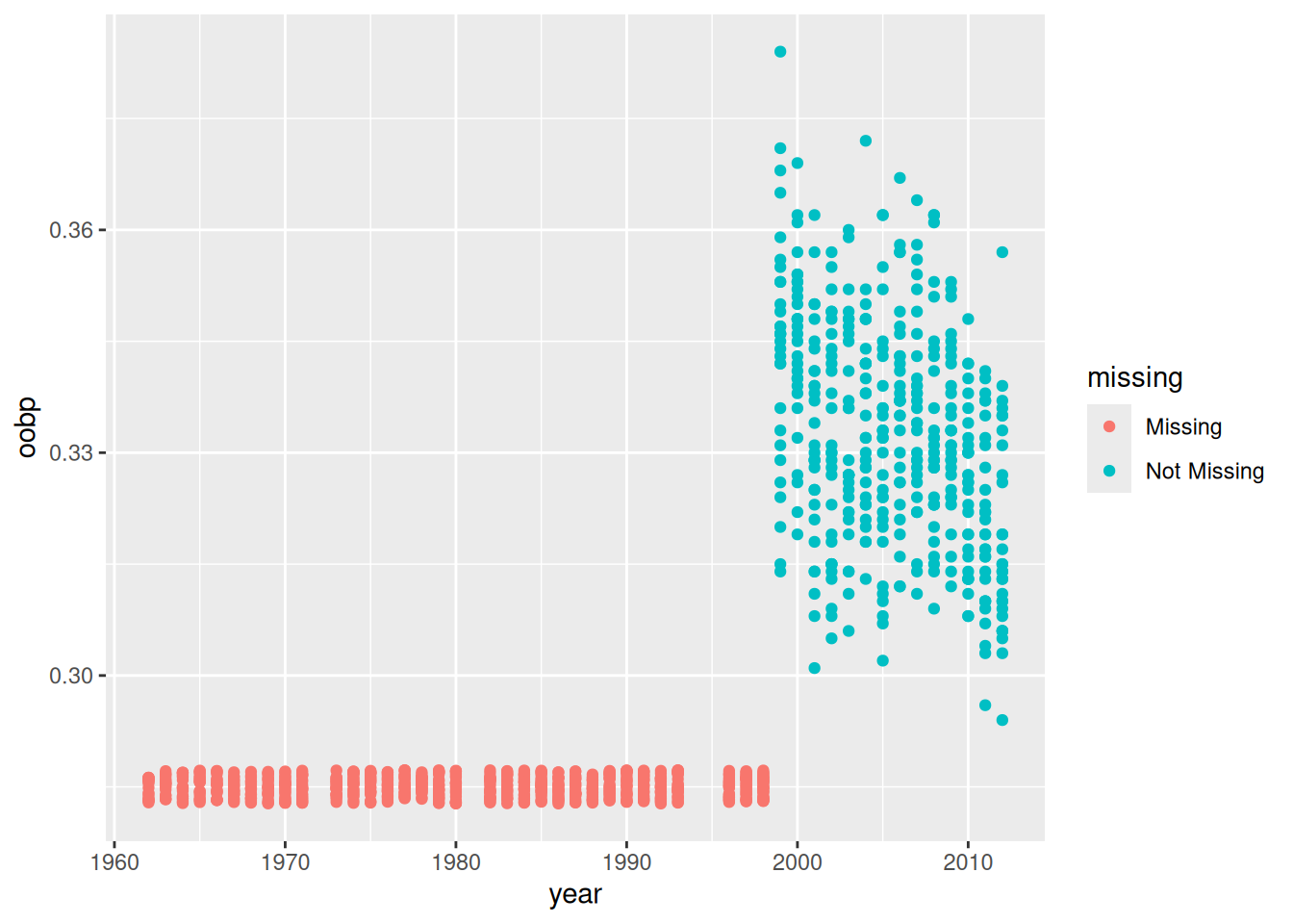

We seem to have a missing data problem. Typically, in this case, we have three options: They are:

Complete case analysis: Exclude all observation with missing values.
Complete feature analysis: Exclude all features with missing values.
Missing value imputation: Use a model to “guess” the missing values (based on the underlying distribution of the data.

Usually, missing value imputation is preferred over the first two. However, in machine learning, one can try out all options and see which performs best for the underlying problem. For now, we limit ourselves to a rather simple imputation technique, imputation by randomly sampling from the univariate distribution. Note that this does not take the multivariate distribution into account properly and that there are more elaborate approaches. We only aim to impute oobp and oslg. For the other missing (categorical) features, we simply add a new level which indicates that information is missing (i.e. all missing values belong to).

It is important to note that in this case here the vast majority of information on the features is missing. In this case, imputation is performed to not throw away the existing information of the features.

mlr3 has some solutions for that within the mlr3pipelines package. We start with an easy PipeOp which only performs numeric imputation.

imp_num = po("imputehist", affect_columns = selector_type(c("integer", "numeric")))

Next, we append the second imputation job for factors.

imp_fct = po("imputeoor", affect_columns = selector_type("factor"))
graph = imp_num %>>% imp_fct
graph$plot(html = FALSE)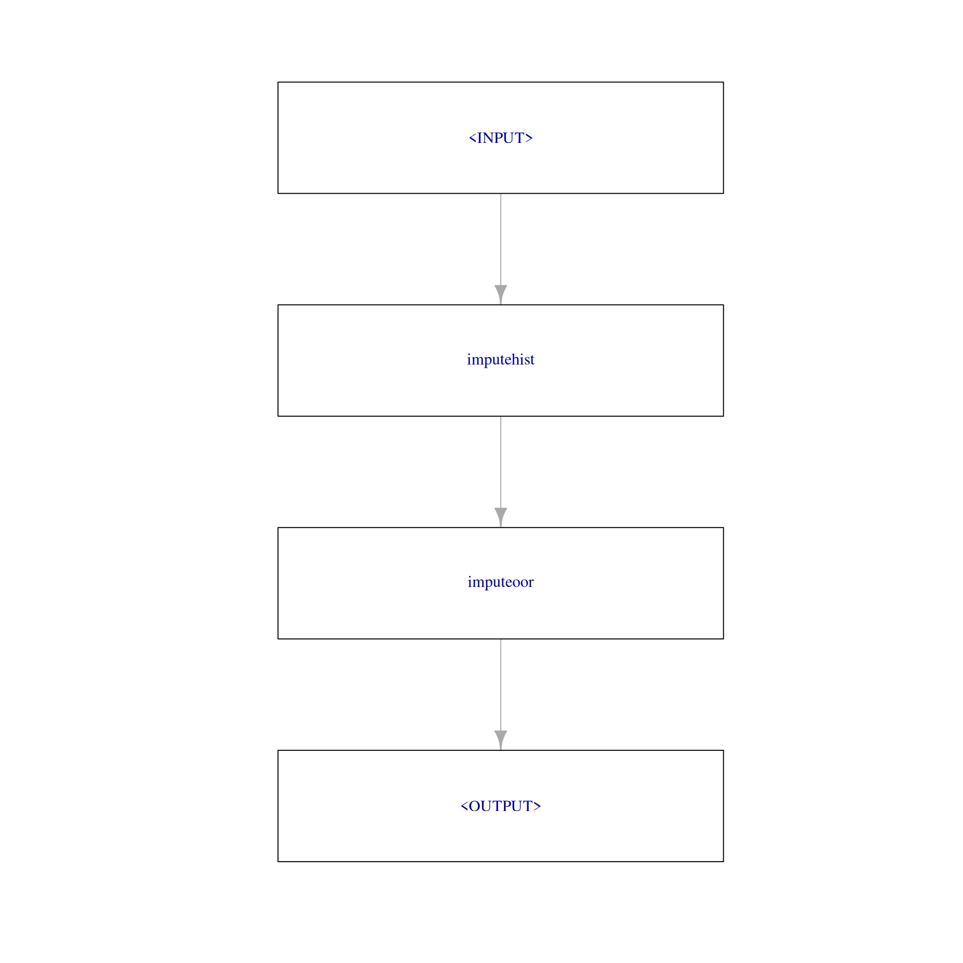

Creating tasks and learners

The fact that there is missing data does not affect the task definition. The task determines what is the problem to be solved by machine learning. We want to explain the runs scored (rs). rs is an important measure as a run is equivalent to a ‘point’ scored in other sports. Naturally, the aim of a coach should be to maximise runs scored and minimise runs allowed. As runs scored and runs allowed are both legitimate targets we ignore the runs allowed here. The task is defined by:

# creates a `mlr3` task from scratch, from a data.frame
# 'target' names the column in the dataset we want to learn to predict
task = as_task_regr(moneyball, target = "rs")
task$missings()

The $missings() method indicates what we already knew: our missing values. Missing values are not always a problem. Some learners can deal with them pretty well. However, we want to use a random forest for our task.

# creates a learner
test_learner = lrn("regr.ranger")

# displays the properties
test_learner$properties

[1] "hotstart_backward" "importance"        "oob_error"         "weights"

Typically, in mlr3 the $properties field would tell us whether missing values are a problem to this learner or not. As it is not listed here, the random forest cannot deal with missing values.

As we aim to use imputation beforehand, we incorporate it into the learner. Our selected learner is going to be a random forest from the ranger package.

One can allow the embedding of the preprocessing (imputation) into a learner by creating a PipeOpLearner. This special Learner can be put into a graph together with the imputer.

# convert learner to pipeop learner and set hyperparameter
pipeop_learner = po(lrn("regr.ranger"), num.trees = 1000, importance = "permutation")

# add pipeop learner to graph and create graph learner
graph_learner = as_learner(graph %>>% pipeop_learner)

The final graph looks like the following:

graph_learner$graph$plot(html = FALSE)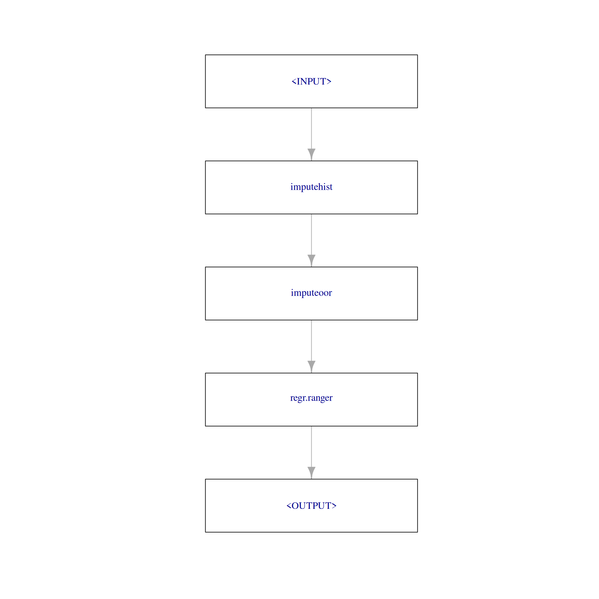

Train and predict

To get a feeling of how our model performs we simply train the Learner on a subset of the data and predict the hold-out data.

# defines the training and testing data; 95% is used for training
train_set = sample(task$nrow, 0.95 * task$nrow)
test_set = setdiff(seq_len(task$nrow), train_set)

# train learner on subset of task
graph_learner$train(task, row_ids = train_set)

# predict using held out observations
prediction = graph_learner$predict(task, row_ids = test_set)

head(as.data.table(prediction))

Viewing the predicted values it seems like the model predicts reasonable values that are fairly close to the truth.

Evaluation & Resampling

While the prediction indicated that the model is doing what it is supposed to, we want to have a more systematic understanding of the model performance. That means we want to know by how much our model is away from the truth on average. Cross-validation investigates this question. In mlr3 10-fold cross-validation is constructed as follows:

cv10 = rsmp("cv", folds = 10)
rr = resample(task, graph_learner, cv10)

We choose some of the performance measures provided by:

as.data.table(mlr_measures)

We choose the mean absolute error and the mean squared error.

rr$score(msrs(c("regr.mae", "regr.mse")))

We can also compute now by how much our model was on average wrong when predicting the runs scored.

rr$aggregate(msr("regr.mae"))

regr.mae 
19.39997

That seems not too bad. Considering that on average approximately 715 runs per team per season have been scored.

mean(moneyball$rs)

[1] 715.082

Performance boost of imputation

To assess if imputation was beneficial, we can compare our current learner with a learner which ignores the missing features. Normally, one would set up a benchmark for this. However, we want to keep things short in this use case. Thus, we only set up the alternative learner (with identical hyperparameters) and compare the 10-fold cross-validated mean absolute error.

As we are mostly interested in the numeric imputation we leave the remaining graph as it is.

impute_oor = po("imputeoor", affect_columns = selector_type("factor"))

Subsequently, we create a pipeline with PipeOpSelect.

feature_names = colnames(moneyball)[!sapply(moneyball, anyNA)]
feature_names = c(feature_names[feature_names %in% task$feature_names],
  "rankseason", "rankplayoffs")
select_na = po("select", selector = selector_name(feature_names))

graph_2 = impute_oor %>>% select_na
graph_2$plot(html = FALSE)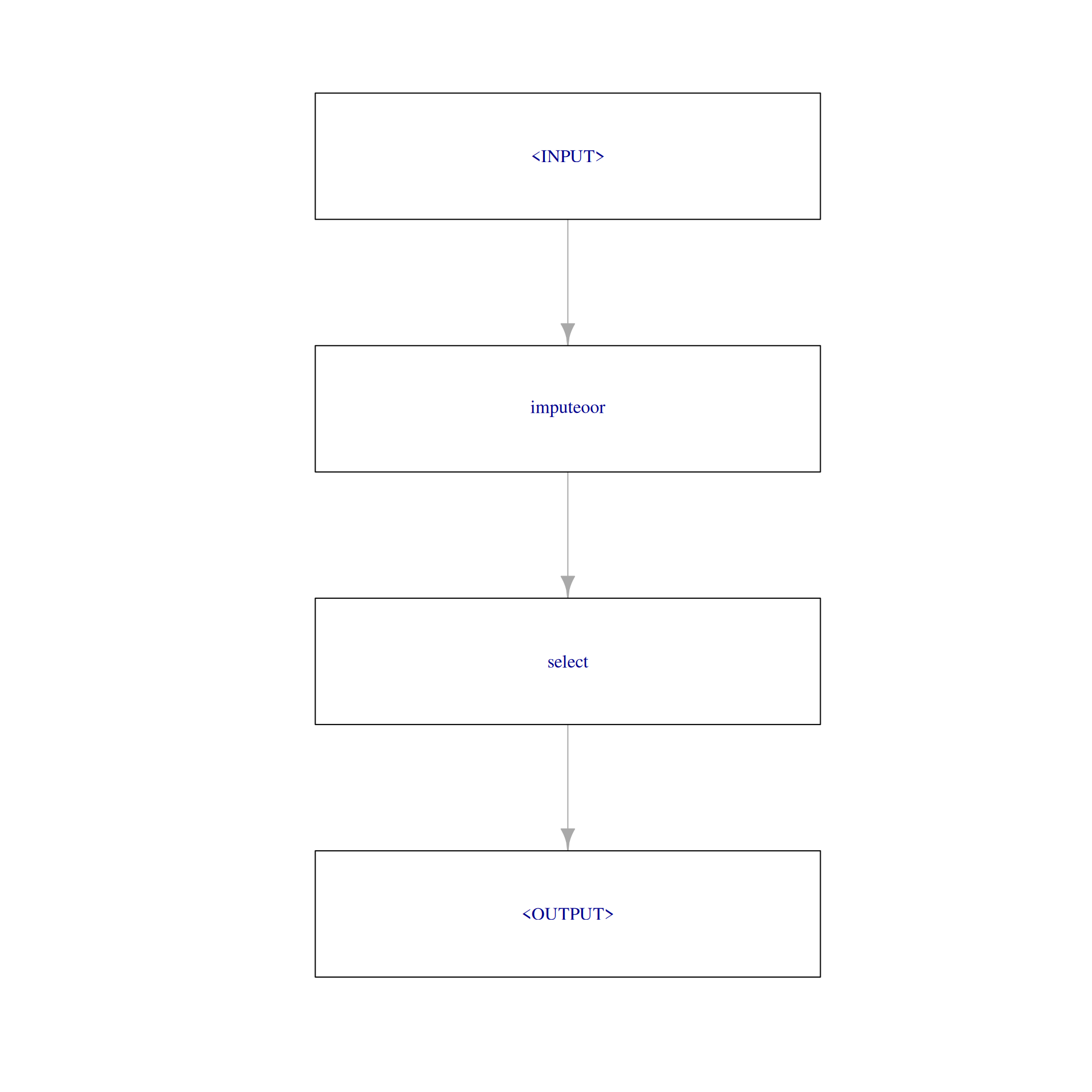

Now we complete the learner and apply resampling as before.

graph_learner_2 = as_learner(graph_2 %>>% pipeop_learner)
rr_2 = resample(task, graph_learner_2, cv10)
rr_2$aggregate(msr("regr.mae"))

regr.mae 
19.03752

Surprisingly, the performance seems to be approximately the same. That means that the imputed features seem not very helpful. We can use the variable.importance of the random forest.

sort(graph_learner$model$regr.ranger$model$variable.importance, decreasing = TRUE)

We see that according to this the left out oobp and oslg seem to have solely rudimentary explanatory power. This may be because there were simply too many instances or because the features are themselves not very powerful.

Conclusion

So, to sum up, what we have learned: We can access very cool data straight away with the OpenML package. (We are working on a better direct implementation into mlr3 at the moment.) We can work with missing data very well in mlr3. Nevertheless, we discovered that sometimes imputation does not lead to the intended goals. We also learned how to use some PipeOps from the mlr3pipelines package.

But most importantly, we found a way to predict the runs scored of MLB teams.

If you want to know more, read the mlr3book and the documentation of the mentioned packages.