%%{ init: { 'flowchart': { 'curve': 'bump' } } }%%

flowchart LR
    subgraph files[Files]
    vector[Vector]
    raster[Raster]
    end
    subgraph load[Load Data]
    sf
    terra
    end
    vector --> sf
    raster --> terra
    subgraph train_model[Train Model]
    task[Task]
    learner[Learner]
    end
    terra --> prediction_raster
    task --> learner
    sf --> task
    subgraph predict[Spatial Prediction]
    prediction_raster[Raster Image]
    end
    learner --> prediction_raster
Scope
Working with spatial data in R requires a lot of data wrangling e.g. reading from different file formats, converting between spatial formats, creating tables from point layers, and predicting spatial raster images. The goal of mlr3spatial is to simplify these workflows within the mlr3 ecosystem. As a practical example, we will perform a land cover classification for the city of Leipzig, Germany. Figure 1 illustrates the typical workflow for this type of task: Load the training data, create a spatial task, train a learner with it, and predict the final raster image.
We assume that you are familiar with the mlr3 ecosystem and know the basic concepts of remote sensing. If not, we recommend reading the mlr3book first. If you are interested in spatial resampling, check out the book chapter on spatial analysis.
Land Cover Classification
Land cover is the physical material or vegetation that covers the surface of the earth, including both natural and human-made features. Understanding land cover patterns and changes over time is critical for addressing global environmental challenges, such as climate change, land degradation, and loss of biodiversity. Land cover classification is the process of assigning land cover classes to pixels in a raster image. With mlr3spatial, we can easily perform a land cover classification within the mlr3 ecosystem.
Before we can start the land cover classification, we need to load the necessary packages. The mlr3spatial package relies on terra for processing raster data and sf for vector data. These widely used packages read all common raster and vector formats. Additionally, the stars and raster packages are supported.
library(mlr3)
library(mlr3spatial)
library(terra, exclude = "resample")
library(sf)
We will work with a Sentinel-2 scene of the city of Leipzig which consists of 7 bands with a 10 or 20m spatial resolution and an NDVI band. The data is included in the mlr3spatial package. We use the terra::rast() to load the TIFF raster file.
leipzig_raster = rast(system.file("extdata", "leipzig_raster.tif", package = "mlr3spatial"))
leipzig_raster
class : SpatRaster
size : 206, 154, 8 (nrow, ncol, nlyr)
resolution : 10, 10 (x, y)
extent : 731810, 733350, 5692030, 5694090 (xmin, xmax, ymin, ymax)
coord. ref. : WGS 84 / UTM zone 32N (EPSG:32632)
source : leipzig_raster.tif
names : b02, b03, b04, b06, b07, b08, ...
min values : 846, 645, 366, 375, 401, 374, ...
max values : 4705, 4880, 5451, 4330, 5162, 5749, ... The training data is a GeoPackage point layer with land cover labels and spectral features. We load the file and create a simple feature point layer.
leipzig_vector = read_sf(system.file("extdata", "leipzig_points.gpkg", package = "mlr3spatial"), stringsAsFactors = TRUE)
leipzig_vector
Simple feature collection with 97 features and 9 fields
Geometry type: POINT
Dimension: XY
Bounding box: xmin: 731930.5 ymin: 5692136 xmax: 733220.3 ymax: 5693968
Projected CRS: WGS 84 / UTM zone 32N
# A tibble: 97 × 10
b02 b03 b04 b06 b07 b08 b11 ndvi land_cover geom
<dbl> <dbl> <dbl> <dbl> <dbl> <dbl> <dbl> <dbl> <fct> <POINT [m]>
1 903 772 426 2998 4240 4029 1816 0.809 forest (732480.1 5693957)
2 1270 1256 1081 1998 2493 2957 2073 0.465 urban (732217.4 5692769)
3 1033 996 777 2117 2748 2799 1595 0.565 urban (732737.2 5692469)
4 962 773 500 465 505 396 153 -0.116 water (733169.3 5692777)
5 1576 1527 1626 1715 1745 1768 1980 0.0418 urban (732202.2 5692644)
6 1125 1185 920 3058 3818 3758 2682 0.607 pasture (732153 5693059)
7 880 746 424 2502 3500 3397 1469 0.778 forest (731937.9 5693722)
8 1332 1251 1385 1663 1799 1640 1910 0.0843 urban (732416.2 5692324)
9 940 741 475 452 515 400 139 -0.0857 water (732933.7 5693344)
10 902 802 454 2764 3821 3666 1567 0.780 forest (732411.3 5693352)
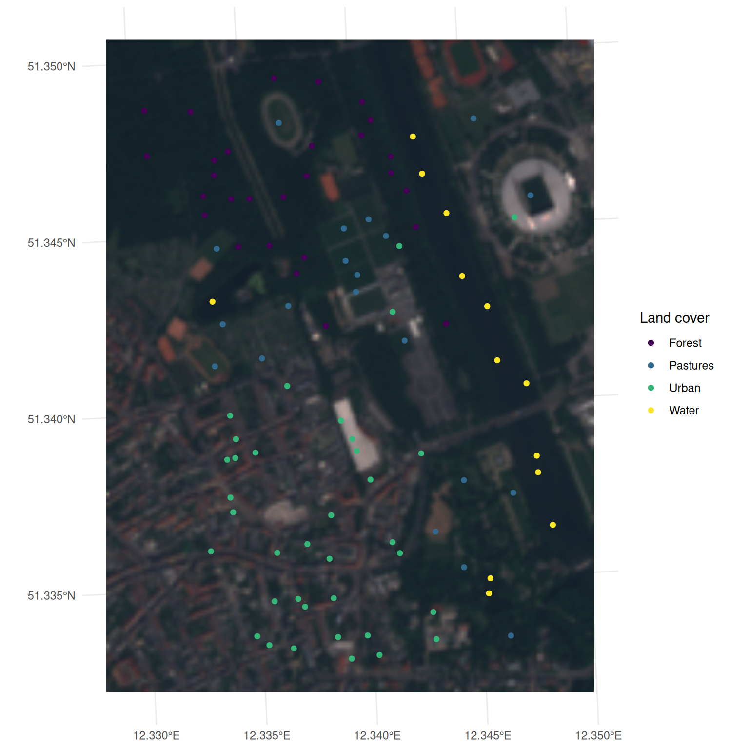
# ℹ 87 more rowsWe plot both layers to get an overview of the data. The training points are located in the districts of Lindenau and Zentrum West.
Code
library(ggplot2)
library(tidyterra, exclude = "filter")

ggplot() +
  geom_spatraster_rgb(data = leipzig_raster, r = 3, g = 2, b = 1, max_col_value = 5451) +
  geom_spatvector(data = leipzig_vector, aes(color = land_cover)) +
  scale_color_viridis_d(name = "Land cover", labels = c("Forest", "Pastures", "Urban", "Water")) +
  theme_minimal()
The as_task_classif_st() function directly creates a spatial task from the point layer. This makes it unnecessary to transform the point layer to a data.frame with coordinates. Spatial tasks additionally store the coordinates of the training points. The coordinates are useful when estimating the performance of the model with spatial resampling.
task = as_task_classif_st(leipzig_vector, target = "land_cover")
task
── <TaskClassifST> (97x9) ──────────────────────────────────────────────────────────────────────────────────────────────
• Target: land_cover
• Properties: multiclass
• Features (8):
  • dbl (8): b02, b03, b04, b06, b07, b08, b11, ndvi
* Coordinates:
           X       Y
       <num>   <num>
 1: 732480.1 5693957
 2: 732217.4 5692769
 3: 732737.2 5692469
 4: 733169.3 5692777
 5: 732202.2 5692644
---
93: 733018.7 5692342
94: 732551.4 5692887
95: 732520.4 5692589
96: 732542.2 5692204
97: 732437.8 5692300
Now we can train a model with the task. We use a simple decision tree learner from the rpart package. The "classif_st" task is a specialization of the "classif" task and therefore works with all "classif" learners.
learner = lrn("classif.rpart")
learner$train(task)
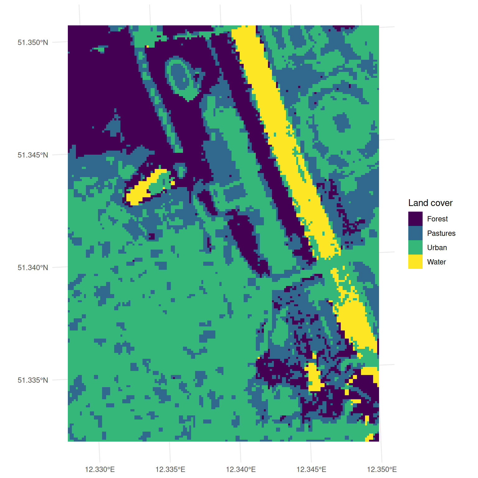
To get a complete land cover classification of Leipzig, we have to predict on each pixel and return a raster image with these predictions. The $predict() method of the learner only works for tabular data. To predict a raster image, we use the predict_spatial() function.
# predict land cover map
land_cover = predict_spatial(leipzig_raster, learner)
Code
ggplot() +
  geom_spatraster(data = land_cover) +
  scale_fill_viridis_d(name = "Land cover", labels = c("Forest", "Pastures", "Urban", "Water")) +
  theme_minimal()
Conclusion
Working with spatial data in R is very easy with the mlr3spatial package. You can quickly train a model with a point layer and predict a raster image. The mlr3spatial package is still in development and we are looking forward to your feedback and contributions.
Session Information
sessioninfo::session_info(info = "packages")═ Session info ═══════════════════════════════════════════════════════════════════════════════════════════════════════
─ Packages ───────────────────────────────────────────────────────────────────────────────────────────────────────────
package * version date (UTC) lib source
backports 1.5.0 2024-05-23 [1] RSPM
checkmate 2.3.4 2026-02-03 [1] RSPM
class 7.3-23 2025-01-01 [2] CRAN (R 4.5.2)
classInt 0.4-11 2025-01-08 [1] RSPM
cli 3.6.5 2025-04-23 [1] RSPM
codetools 0.2-20 2024-03-31 [2] CRAN (R 4.5.2)
crayon 1.5.3 2024-06-20 [1] RSPM
data.table * 1.18.2.1 2026-01-27 [1] RSPM
DBI 1.3.0 2026-02-25 [1] RSPM
digest 0.6.39 2025-11-19 [1] RSPM
dplyr 1.2.0 2026-02-03 [1] RSPM
e1071 1.7-17 2025-12-18 [1] RSPM
evaluate 1.0.5 2025-08-27 [1] RSPM
farver 2.1.2 2024-05-13 [1] RSPM
fastmap 1.2.0 2024-05-15 [1] RSPM
future 1.69.0 2026-01-16 [1] RSPM
generics 0.1.4 2025-05-09 [1] RSPM
ggplot2 * 4.0.2 2026-02-03 [1] RSPM
globals 0.19.0 2026-02-02 [1] RSPM
glue 1.8.0 2024-09-30 [1] RSPM
gtable 0.3.6 2024-10-25 [1] RSPM
htmltools 0.5.9 2025-12-04 [1] RSPM
htmlwidgets 1.6.4 2023-12-06 [1] RSPM
jsonlite 2.0.0 2025-03-27 [1] RSPM
KernSmooth 2.23-26 2025-01-01 [2] CRAN (R 4.5.2)
knitr 1.51 2025-12-20 [1] RSPM
lgr 0.5.2 2026-01-30 [1] RSPM
lifecycle 1.0.5 2026-01-08 [1] RSPM
listenv 0.10.0 2025-11-02 [1] RSPM
magrittr 2.0.4 2025-09-12 [1] RSPM
mlr3 * 1.4.0 2026-02-19 [1] RSPM
mlr3misc 0.21.0 2026-02-26 [1] RSPM
mlr3spatial * 0.6.1 2025-09-14 [1] RSPM
mlr3website * 0.0.0.9000 2026-02-27 [1] Github (mlr-org/mlr3website@f6e32a7)
otel 0.2.0 2025-08-29 [1] RSPM
palmerpenguins 0.1.1 2022-08-15 [1] RSPM
paradox 1.0.1 2024-07-09 [1] RSPM
parallelly 1.46.1 2026-01-08 [1] RSPM
pillar 1.11.1 2025-09-17 [1] RSPM
pkgconfig 2.0.3 2019-09-22 [1] RSPM
proxy 0.4-29 2025-12-29 [1] RSPM
purrr 1.2.1 2026-01-09 [1] RSPM
R6 2.6.1 2025-02-15 [1] RSPM
RColorBrewer 1.1-3 2022-04-03 [1] RSPM
Rcpp 1.1.1 2026-01-10 [1] RSPM
rlang 1.1.7 2026-01-09 [1] RSPM
rmarkdown 2.30 2025-09-28 [1] RSPM
rpart 4.1.24 2025-01-07 [2] CRAN (R 4.5.2)
S7 0.2.1 2025-11-14 [1] RSPM
scales 1.4.0 2025-04-24 [1] RSPM
sessioninfo 1.2.3 2025-02-05 [1] RSPM
sf * 1.1-0 2026-02-24 [1] RSPM
stringi 1.8.7 2025-03-27 [1] RSPM
terra * 1.8-93 2026-01-12 [1] RSPM
tibble 3.3.1 2026-01-11 [1] RSPM
tidyr 1.3.2 2025-12-19 [1] RSPM
tidyselect 1.2.1 2024-03-11 [1] RSPM
tidyterra * 1.0.0 2026-01-23 [1] RSPM
units 1.0-0 2025-10-09 [1] RSPM
utf8 1.2.6 2025-06-08 [1] RSPM
uuid 1.2-2 2026-01-23 [1] RSPM
vctrs 0.7.1 2026-01-23 [1] RSPM
viridisLite 0.4.3 2026-02-04 [1] RSPM
withr 3.0.2 2024-10-28 [1] RSPM
xfun 0.56 2026-01-18 [1] RSPM
yaml 2.3.12 2025-12-10 [1] RSPM
[1] /usr/local/lib/R/site-library
[2] /usr/local/lib/R/library
* ── Packages attached to the search path.
──────────────────────────────────────────────────────────────────────────────────────────────────────────────────────