
library(mlr3viz)
library(mlr3learners)
library(mlr3tuning)
library(mlr3cluster)

task = tsk("penguins")
task$select(c("body_mass", "bill_length"))

autoplot(task, type = "target")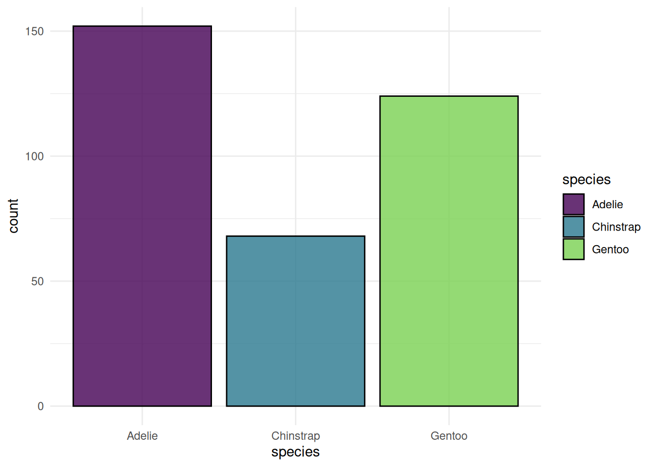
We showcase the visualization functions of the mlr3 ecosystem. The mlr3viz package creates a plot for almost all mlr3 objects. This post displays all available plots with their reproducible code. We start with plots of the base mlr3 objects. This includes boxplots of tasks, dendrograms of cluster learners and ROC curves of predictions. After that, we tune a classification tree and visualize the results. Finally, we show visualizations for filters.
This article will be updated whenever a new plot is available in mlr3viz.
The mlr3viz package defines autoplot() functions to draw plots with ggplot2. Often there is more than one type of plot for an object. You can change the plot with the type argument. The help pages list all possible choices. The easiest way to access the help pages is via the pkgdown website. The plots use the viridis color pallet and the appearance is controlled with the theme argument. By default, the minimal theme is applied.
We begin with plots of the classification task Palmer Penguins. We plot the class frequency of the target variable.
library(mlr3viz)
library(mlr3learners)
library(mlr3tuning)
library(mlr3cluster)
task = tsk("penguins")
task$select(c("body_mass", "bill_length"))
autoplot(task, type = "target")
The "duo" plot shows the distribution of multiple features.
autoplot(task, type = "duo")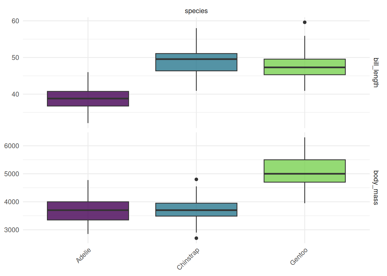
The "pairs" plot shows the pairwise comparison of multiple features. The classes of the target variable are shown in different colors.
autoplot(task, type = "pairs")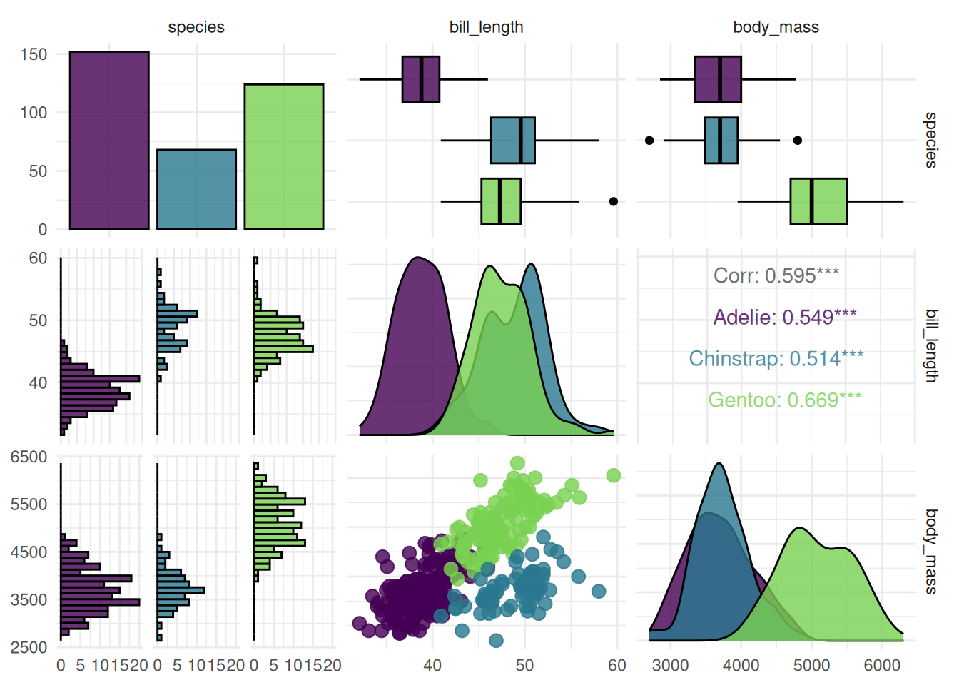
Next, we plot the regression task mtcars. We create a boxplot of the target variable.
task = tsk("mtcars")
task$select(c("am", "carb"))

autoplot(task, type = "target")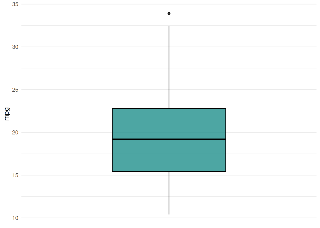
The "pairs" plot shows the pairwise comparison of mutiple features and the target variable.
autoplot(task, type = "pairs")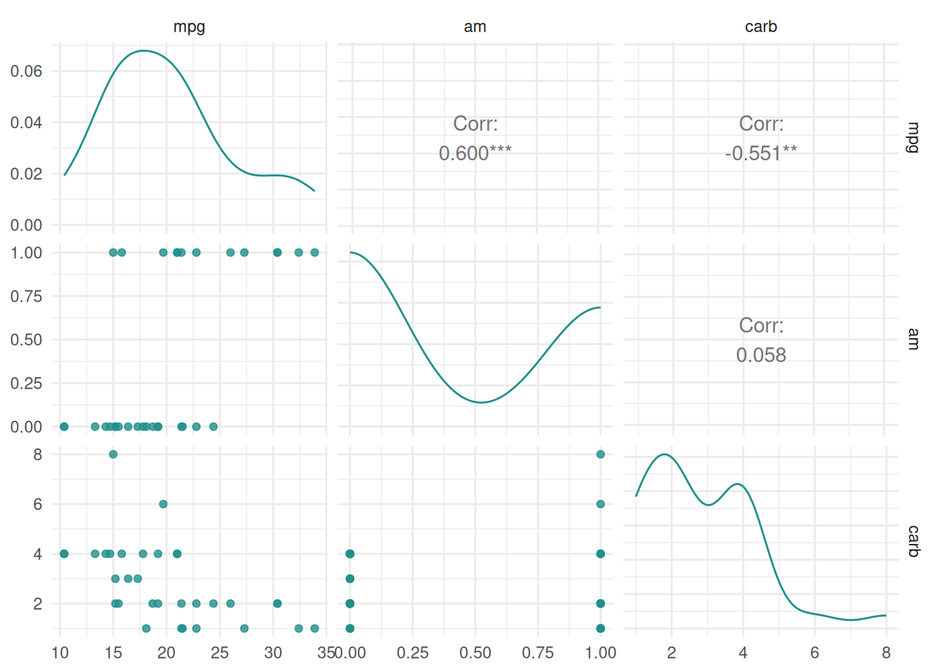
Finally, we plot the cluster task US Arrests. The "pairs" plot shows the pairwise comparison of mutiple features.
library(mlr3cluster)

task = mlr_tasks$get("usarrests")

autoplot(task, type = "pairs")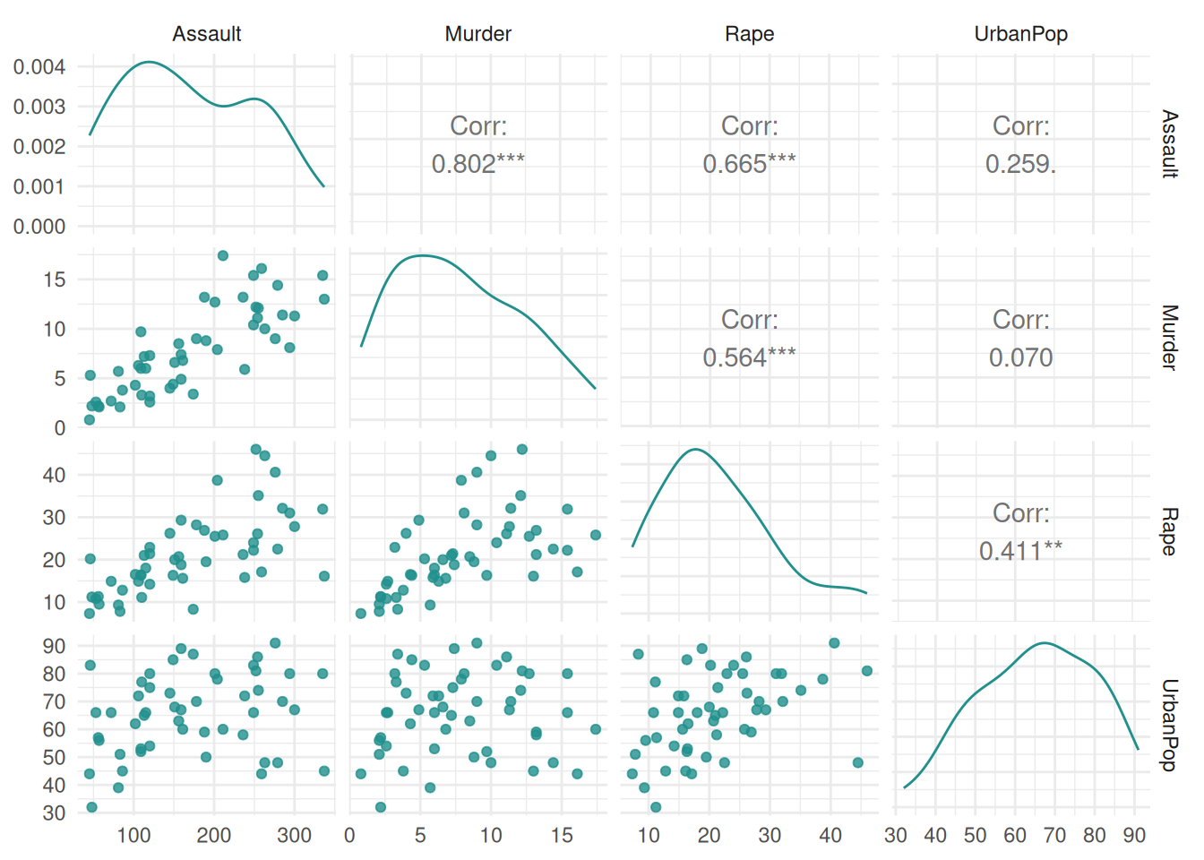
The "prediction" plot shows the decision boundary of a classification learner and the true class labels as points.
task = tsk("diabetes")$select(c("age", "pedigree"))
learner = lrn("classif.rpart")
learner$train(task)

autoplot(learner, type = "prediction", task)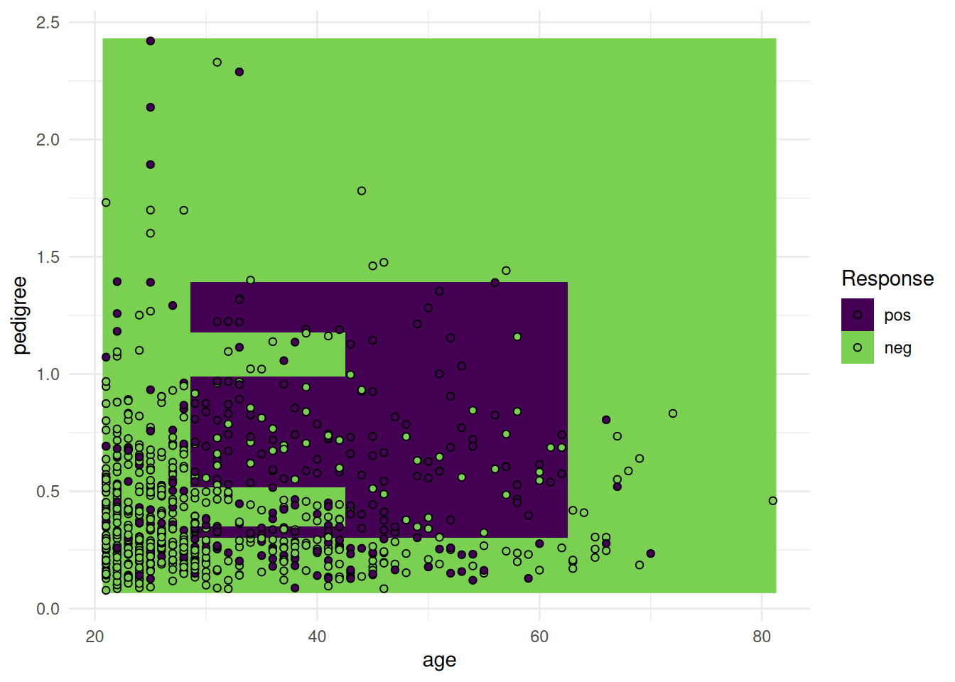
Using probabilities.
task = tsk("diabetes")$select(c("age", "pedigree"))
learner = lrn("classif.rpart", predict_type = "prob")
learner$train(task)

autoplot(learner, type = "prediction", task)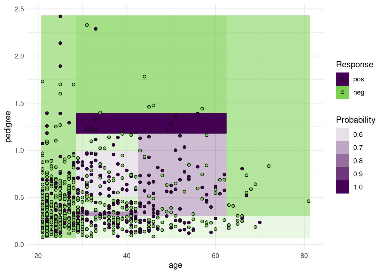
The "prediction" plot of a regression learner illustrates the decision boundary and the true response as points.
task = tsk("california_housing")$select("median_income")
learner = lrn("regr.rpart")
learner$train(task)

autoplot(learner, type = "prediction", task)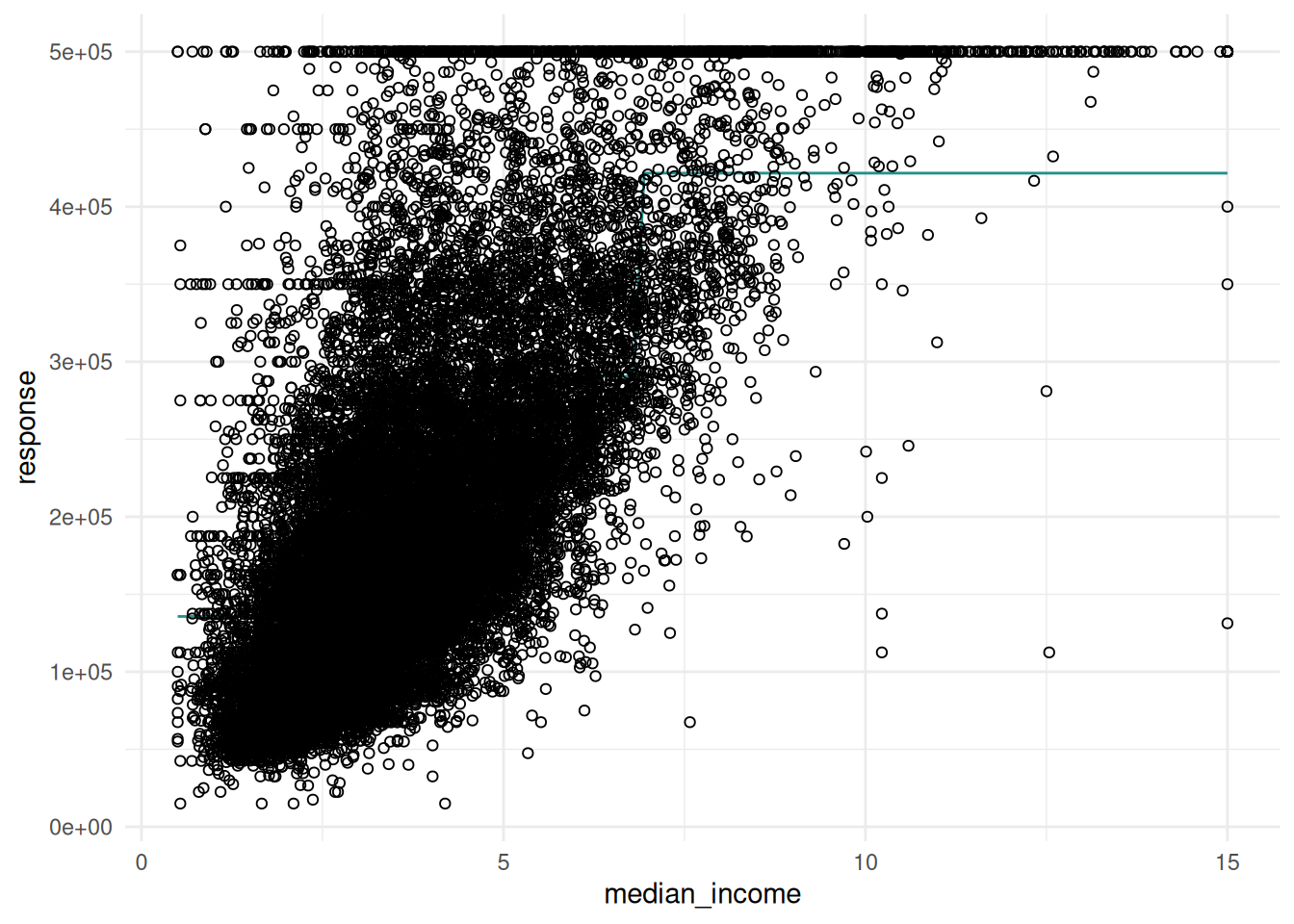
When using two features, the response surface is plotted in the background.
task = tsk("california_housing")$select(c("latitude", "longitude"))
learner = lrn("regr.rpart")
learner$train(task)

autoplot(learner, type = "prediction", task)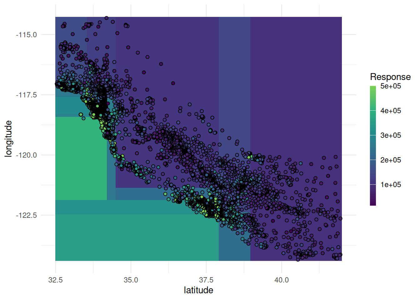
The classification and regression GLMNet learner is equipped with a plot function.
library(mlr3data)

task = tsk("ilpd")
task$select(setdiff(task$feature_names, "gender"))
learner = lrn("classif.glmnet")
learner$train(task)

autoplot(learner, type = "ggfortify")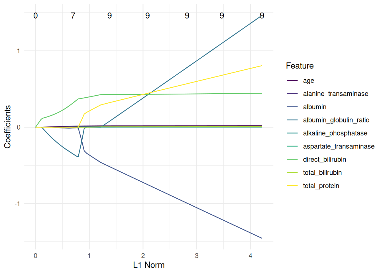
task = tsk("mtcars")
learner = lrn("regr.glmnet")
learner$train(task)

autoplot(learner, type = "ggfortify")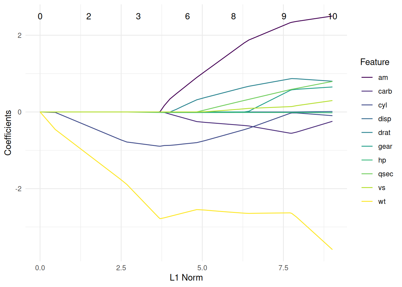
We plot a classification tree of the rpart package. We have to fit the learner with keep_model = TRUE to keep the model object.
task = tsk("penguins")
learner = lrn("classif.rpart", keep_model = TRUE)
learner$train(task)

autoplot(learner, type = "ggparty")
Warning in ggparty::geom_edge_label(): Ignoring unknown parameters: `label.size`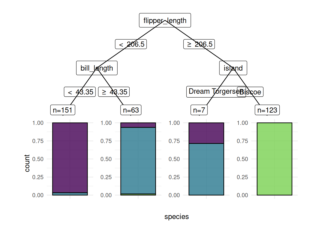
We can also plot regression trees.
task = tsk("mtcars")
learner = lrn("regr.rpart", keep_model = TRUE)
learner$train(task)

autoplot(learner, type = "ggparty")
Warning in ggparty::geom_edge_label(): Ignoring unknown parameters: `label.size`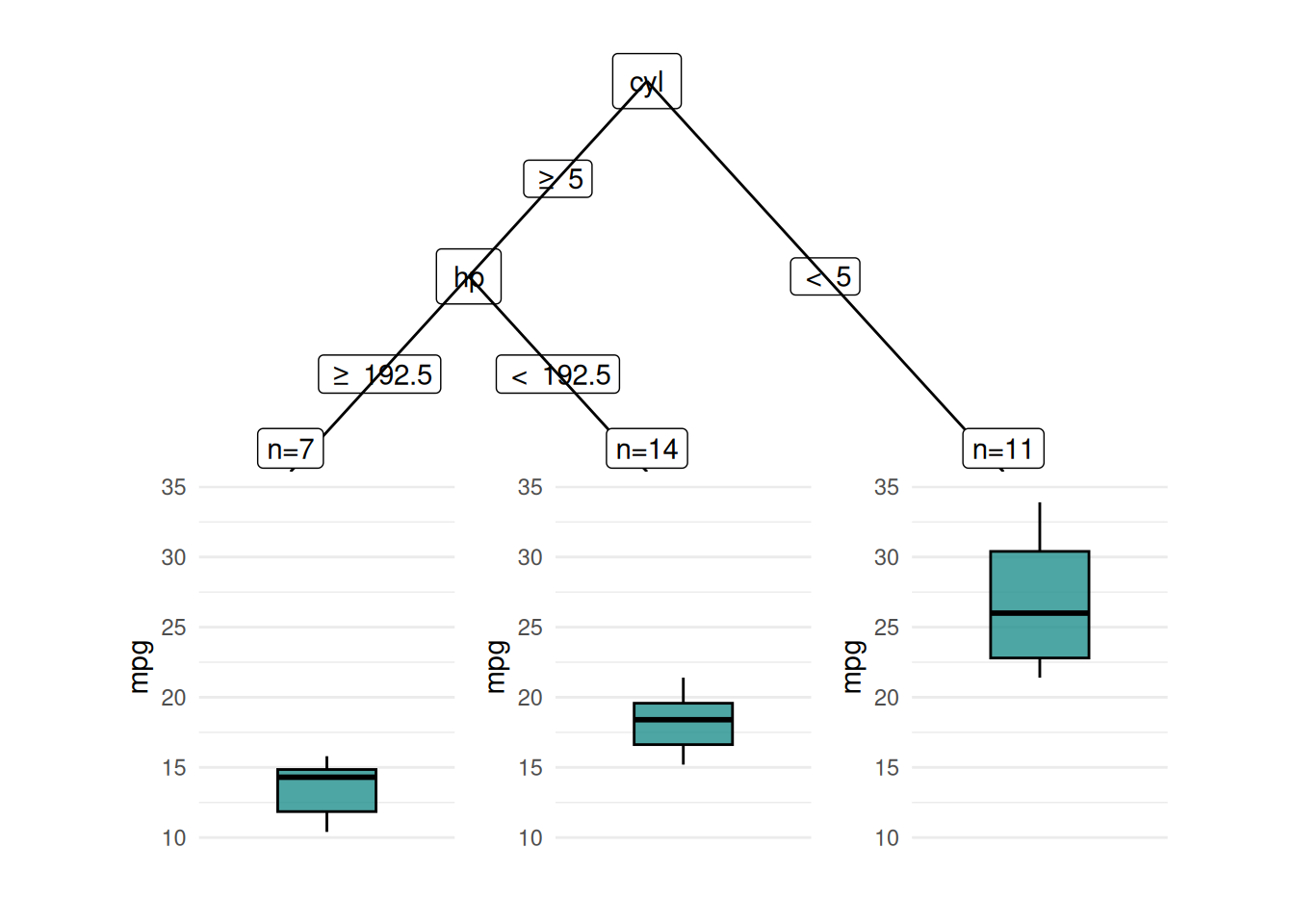
The "dend" plot shows the result of the hierarchical clustering of the data.
library(mlr3cluster)

task = tsk("usarrests")
learner = lrn("clust.hclust")
learner$train(task)

autoplot(learner, type = "dend", task = task)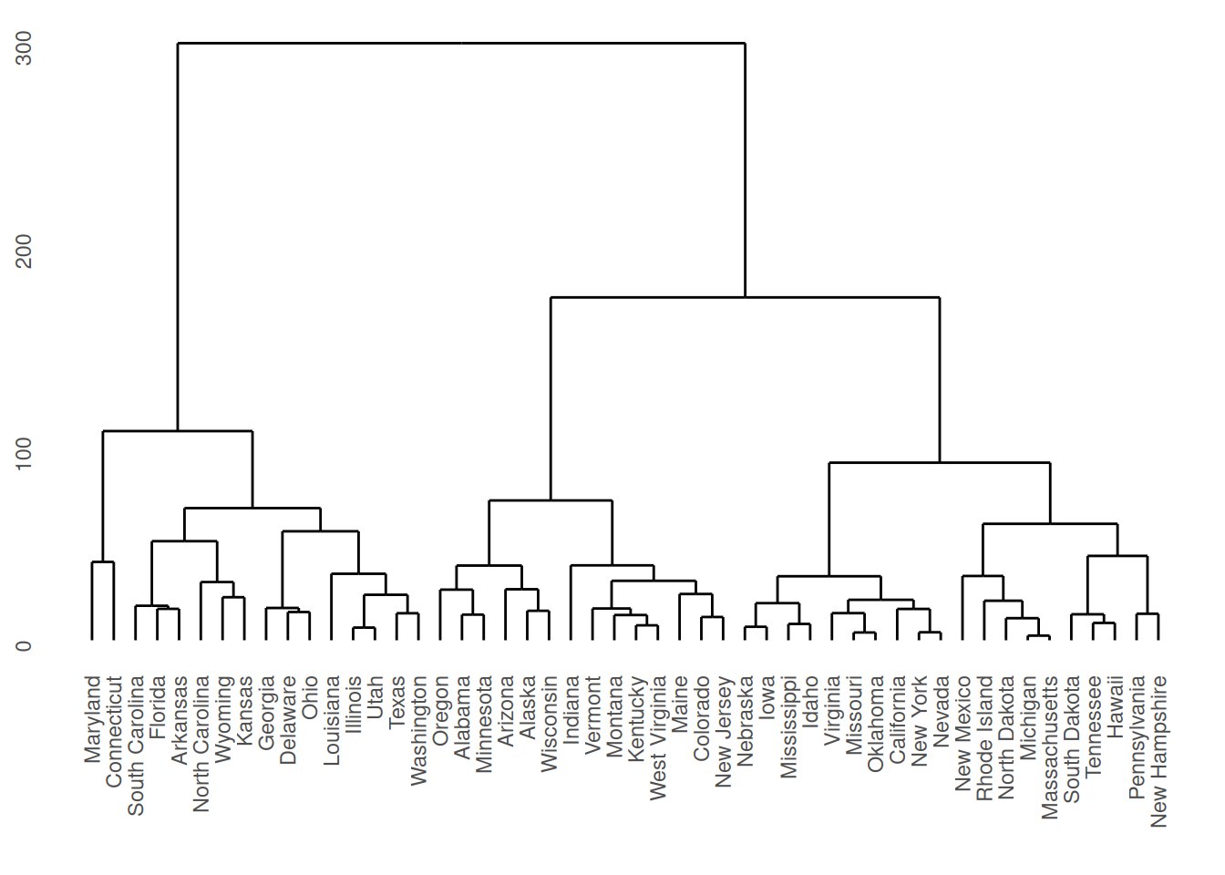
The "scree" type plots the number of clusters and the height.
autoplot(learner, type = "scree")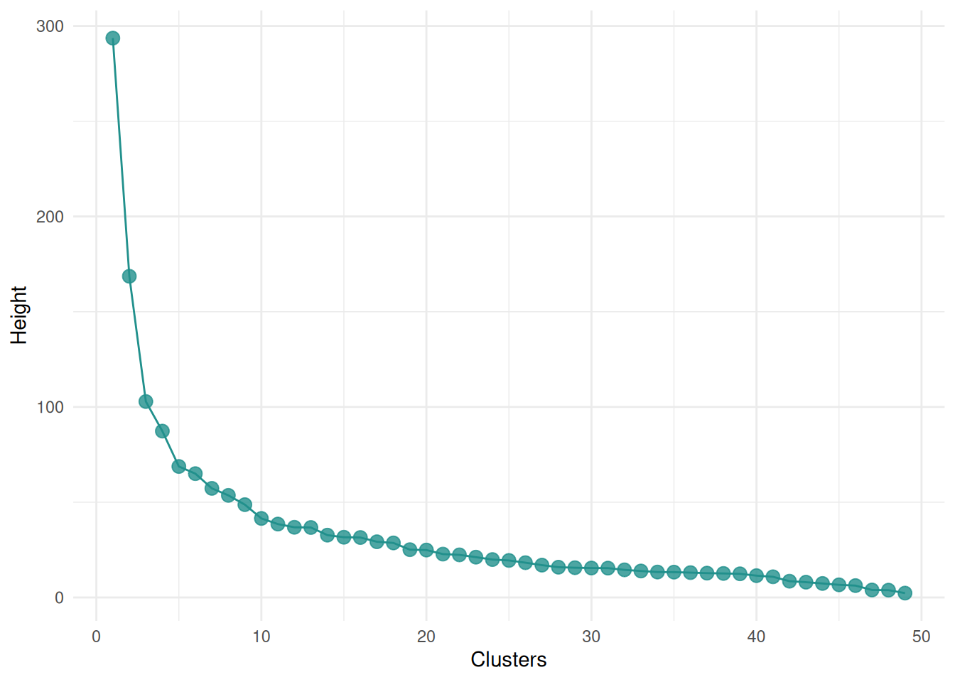
We plot the predictions of a classification learner. The "stacked" plot shows the predicted and true class labels.
task = tsk("spam")
learner = lrn("classif.rpart", predict_type = "prob")
pred = learner$train(task)$predict(task)

autoplot(pred, type = "stacked")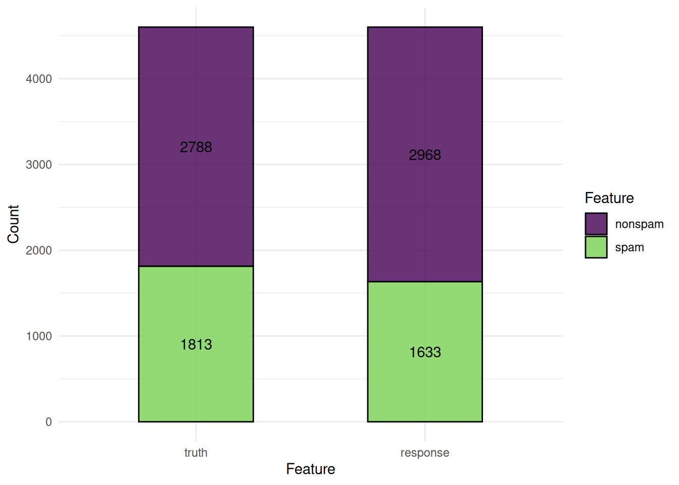
The ROC curve plots the true positive rate against the false positive rate at different thresholds.
autoplot(pred, type = "roc")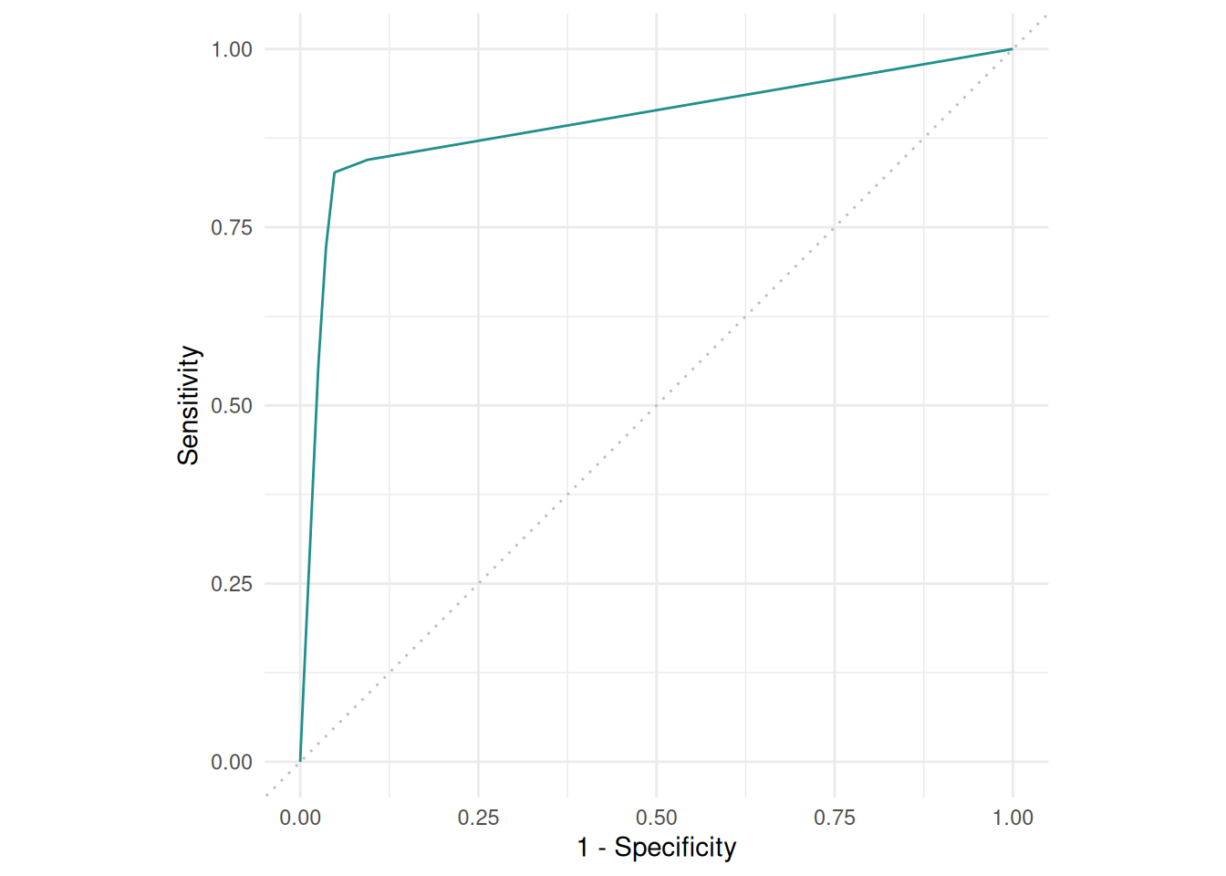
The precision-recall curve plots the precision against the recall at different thresholds.
autoplot(pred, type = "prc")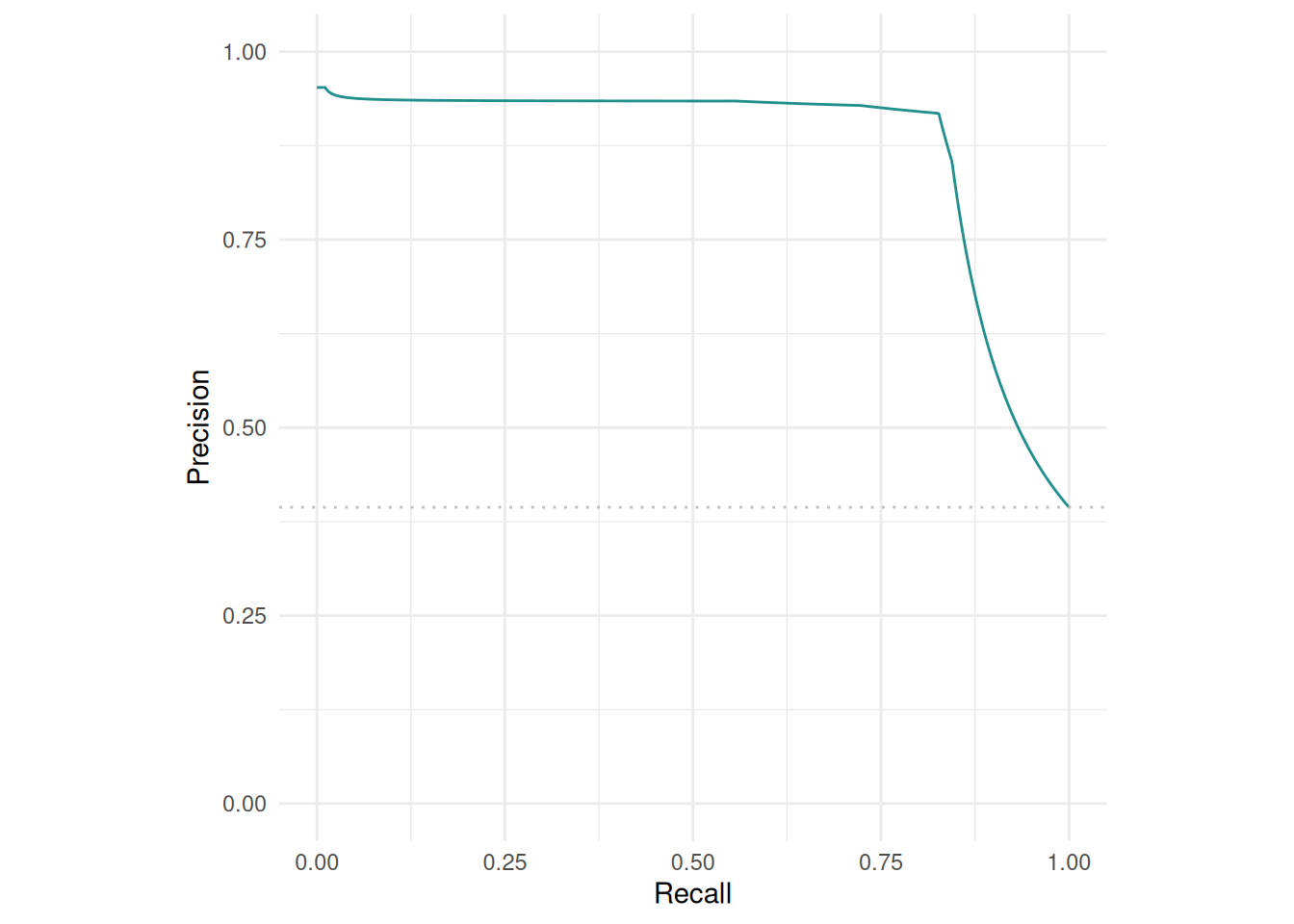
The "threshold" plot varies the threshold of a binary classification and plots against the resulting performance.
autoplot(pred, type = "threshold")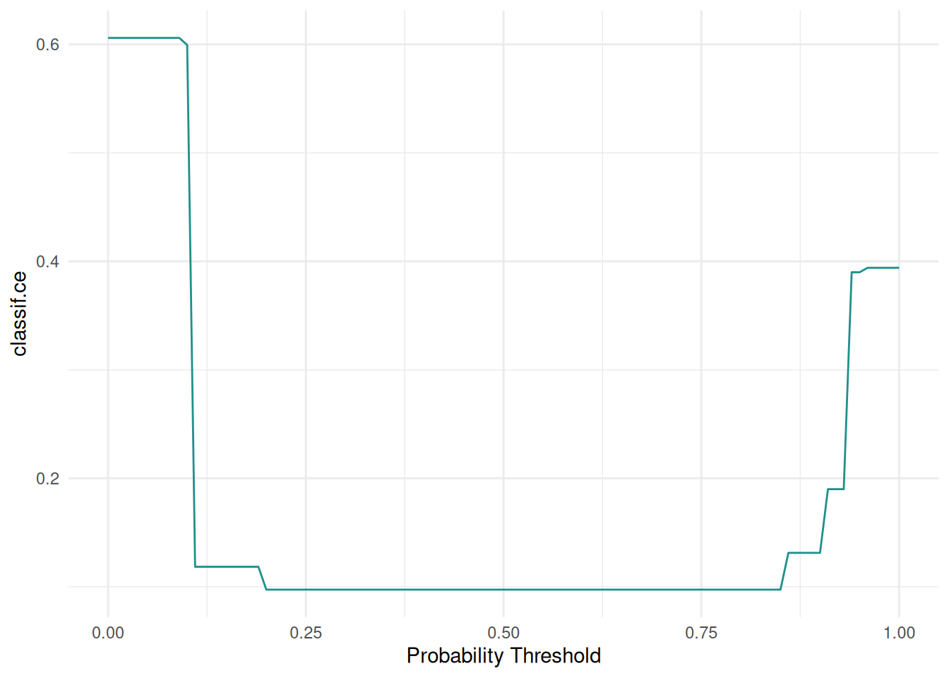
The predictions of a regression learner are often presented as a scatterplot of truth and predicted response.
task = tsk("california_housing")
learner = lrn("regr.rpart")
pred = learner$train(task)$predict(task)

autoplot(pred, type = "xy")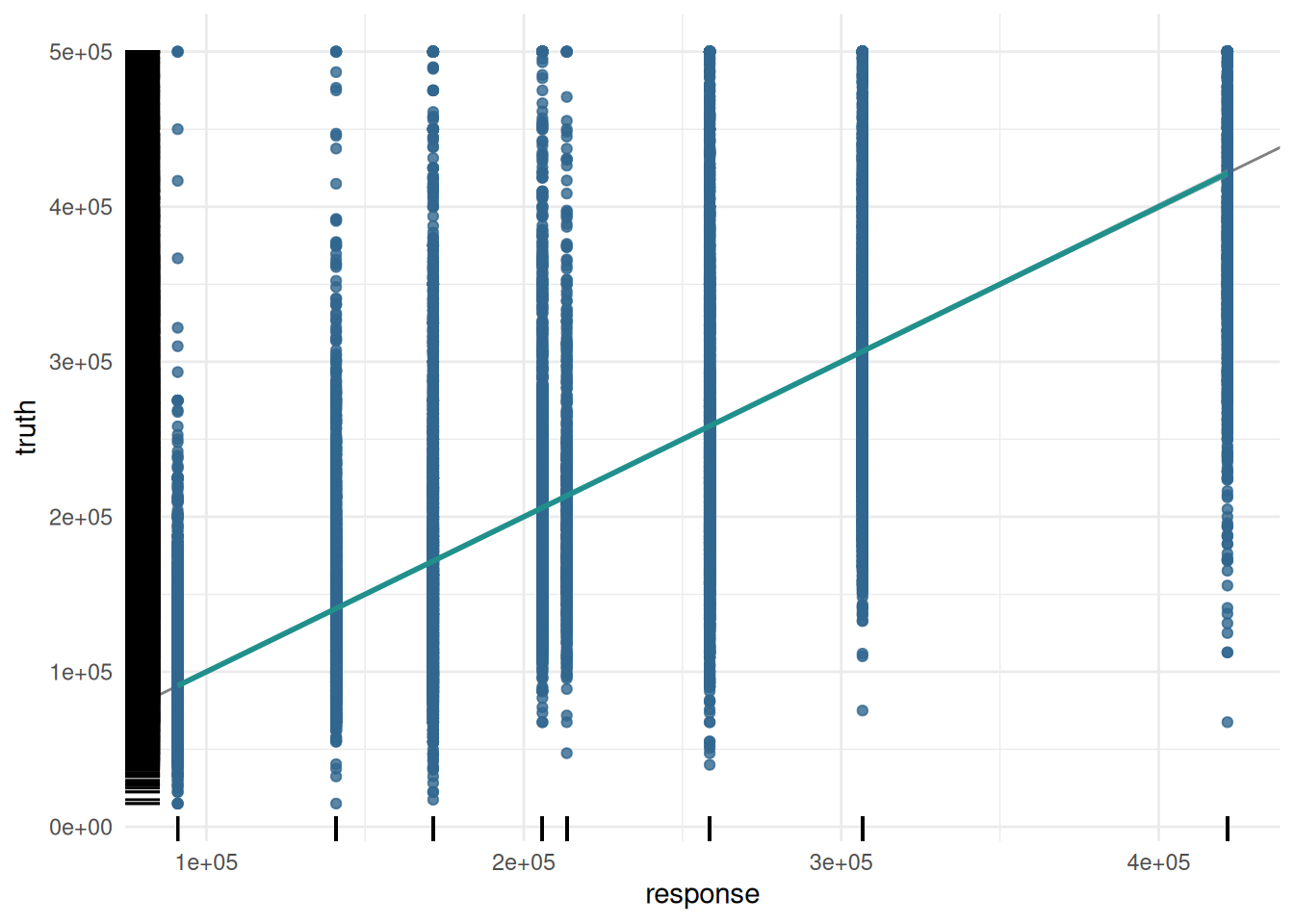
Additionally, we plot the response with the residuals.
autoplot(pred, type = "residual")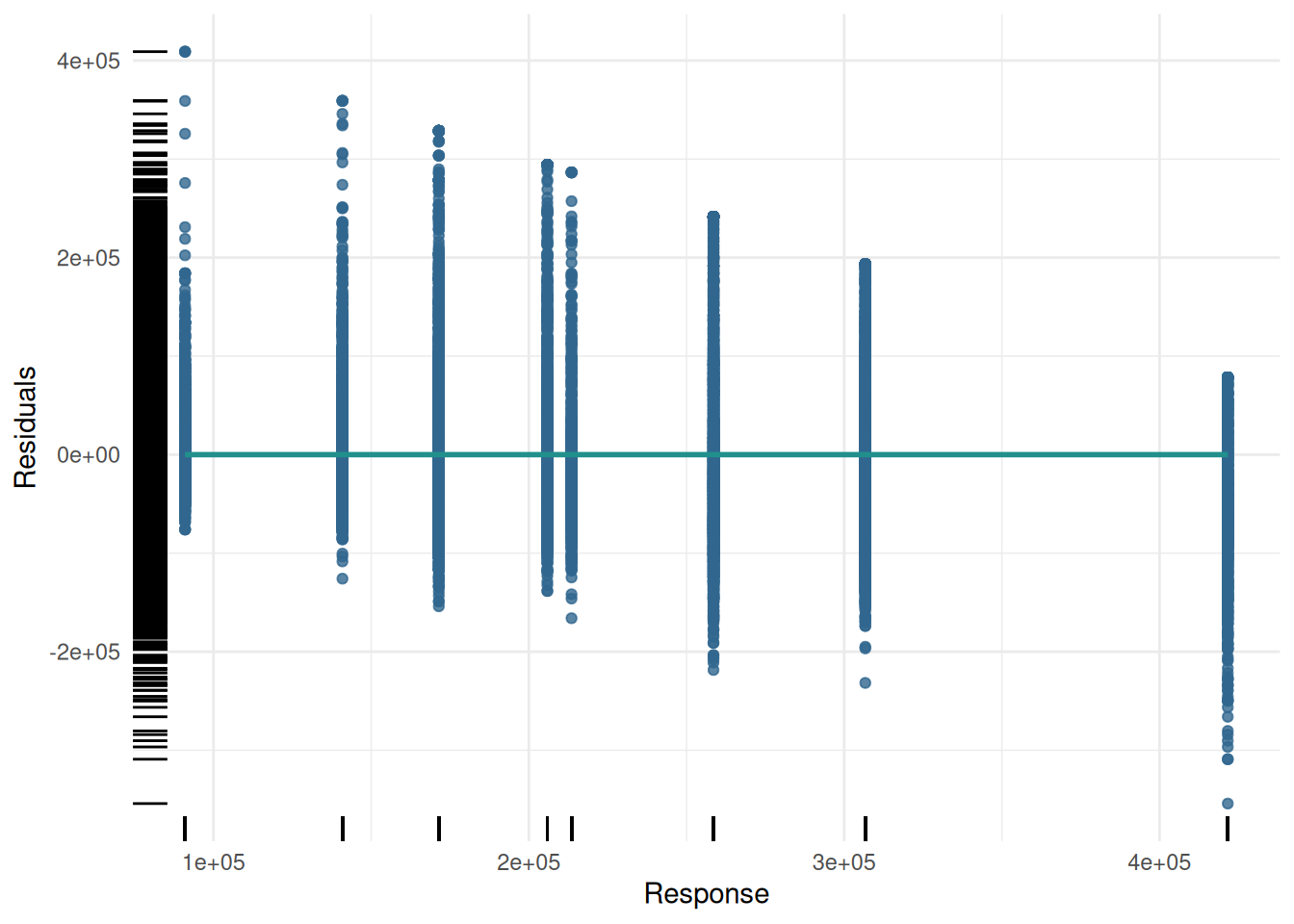
We can also plot the distribution of the residuals.
autoplot(pred, type = "histogram")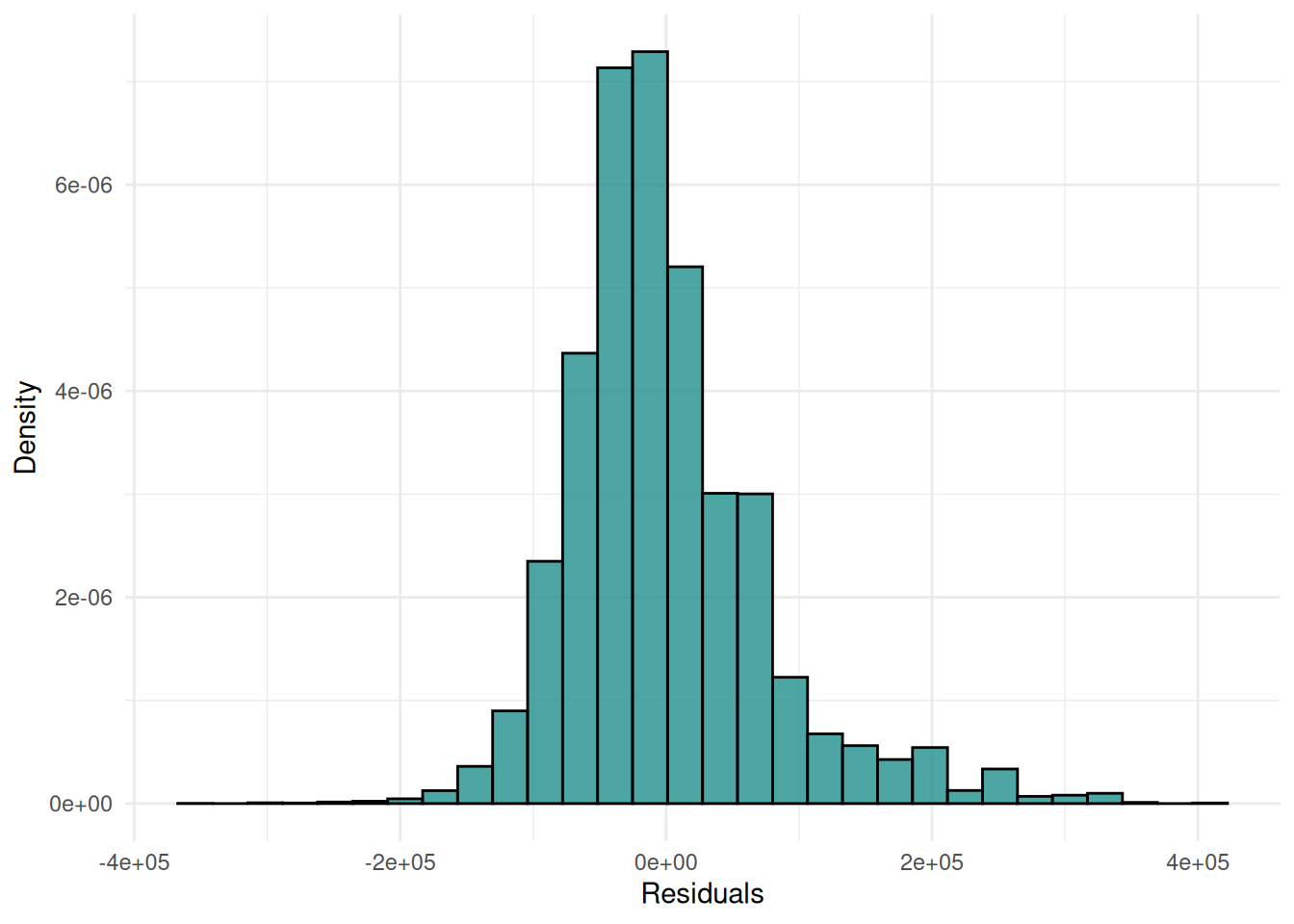
The predictions of a cluster learner are often presented as a scatterplot of the data points colored by the cluster.
library(mlr3cluster)

task = tsk("usarrests")
learner = lrn("clust.kmeans", centers = 3)
pred = learner$train(task)$predict(task)

autoplot(pred, task, type = "scatter")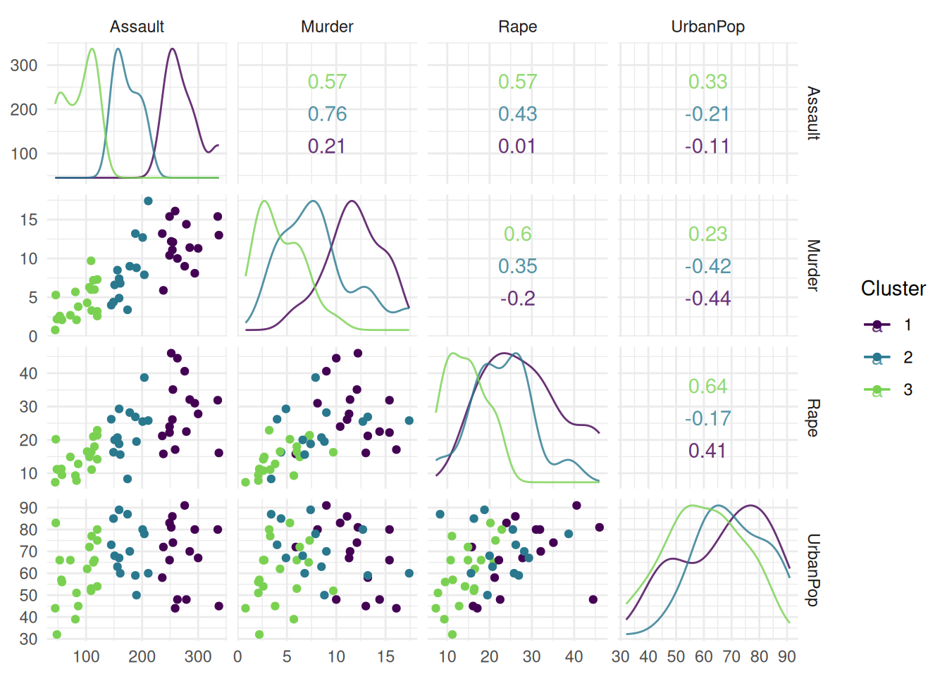
The "sil" plot shows the silhouette width of the clusters. The dashed line is the mean silhouette width.
autoplot(pred, task, type = "sil")Warning: Using `size` aesthetic for lines was deprecated in ggplot2 3.4.0.
ℹ Please use `linewidth` instead.
ℹ The deprecated feature was likely used in the ggfortify package.
Please report the issue at <https://github.com/sinhrks/ggfortify/issues>.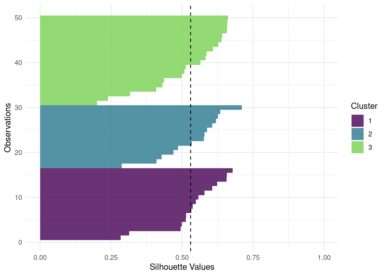
The "pca" plot shows the first two principal components of the data colored by the cluster.
autoplot(pred, task, type = "pca")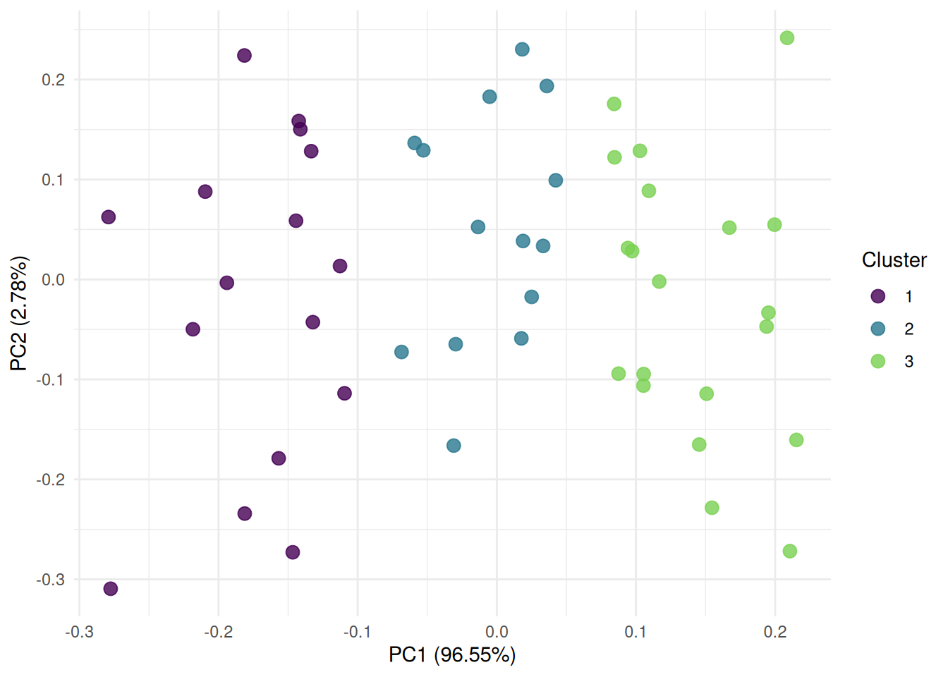
The "boxplot" shows the distribution of the performance measures.
task = tsk("sonar")
learner = lrn("classif.rpart", predict_type = "prob")
resampling = rsmp("cv")
rr = resample(task, learner, resampling)

autoplot(rr, type = "boxplot")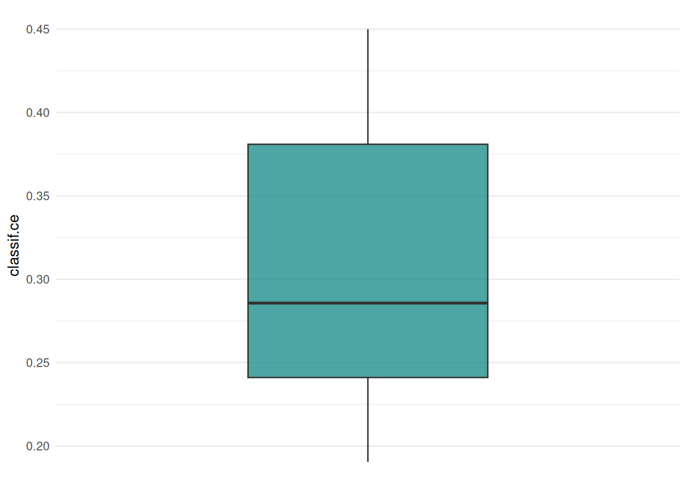
We can also plot the distribution of the performance measures as a “histogram”.
autoplot(rr, type = "histogram")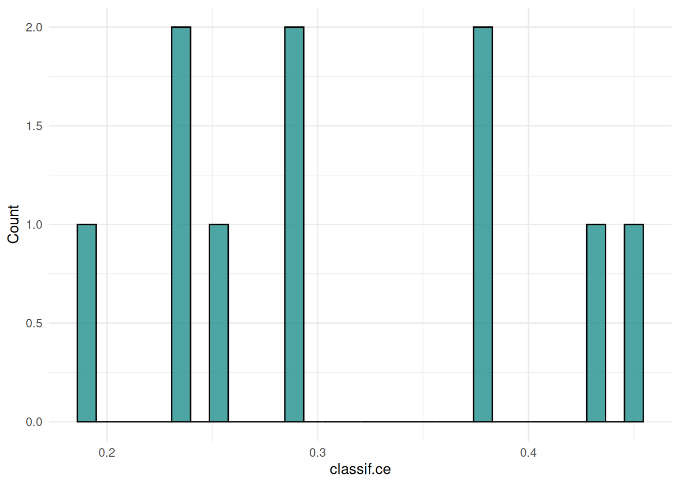
The ROC curve plots the true positive rate against the false positive rate at different thresholds.
autoplot(rr, type = "roc")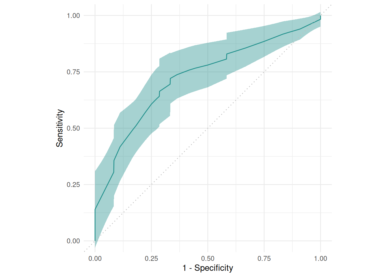
The precision-recall curve plots the precision against the recall at different thresholds.
autoplot(rr, type = "prc")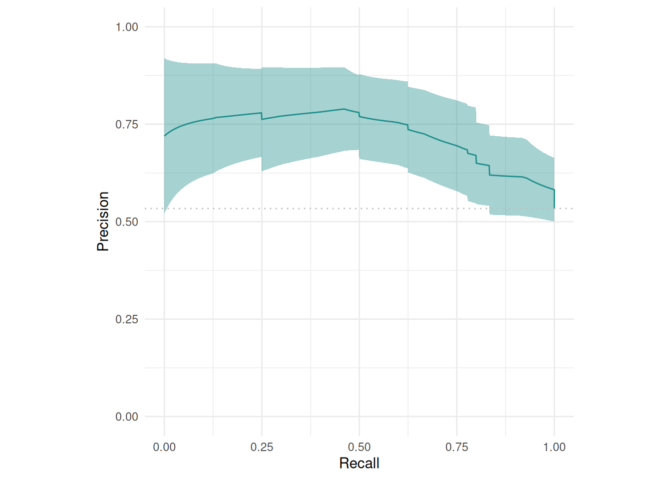
The "prediction" plot shows two features and the predicted class in the background. Points mark the observations of the test set and the color presents the truth.
task = tsk("diabetes")
task$filter(seq(100))
task$select(c("age", "glucose"))
learner = lrn("classif.rpart")
resampling = rsmp("cv", folds = 3)
rr = resample(task, learner, resampling, store_models = TRUE)

autoplot(rr, type = "prediction")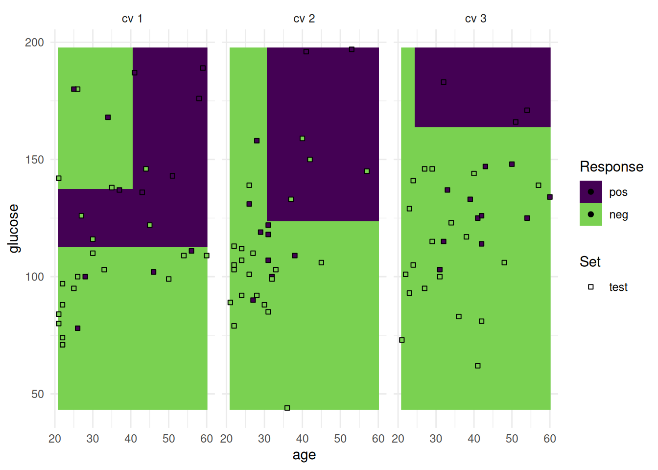
Alternatively, we can plot class probabilities.
task = tsk("diabetes")
task$filter(seq(100))
task$select(c("age", "glucose"))
learner = lrn("classif.rpart", predict_type = "prob")
resampling = rsmp("cv", folds = 3)
rr = resample(task, learner, resampling, store_models = TRUE)

autoplot(rr, type = "prediction")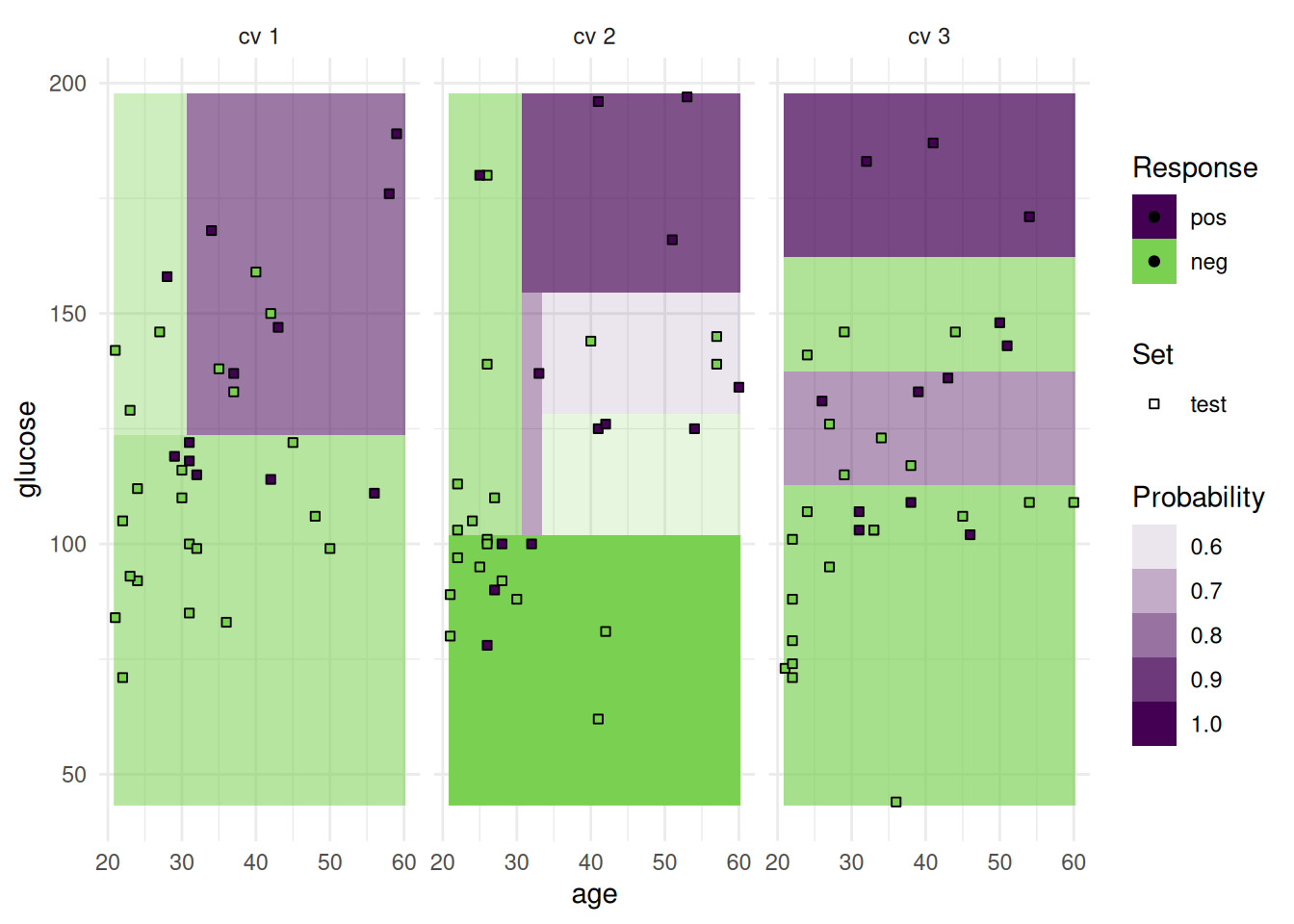
In addition to the test set, we can also plot the train set.
task = tsk("diabetes")
task$filter(seq(100))
task$select(c("age", "glucose"))
learner = lrn("classif.rpart", predict_type = "prob", predict_sets = c("train", "test"))
resampling = rsmp("cv", folds = 3)
rr = resample(task, learner, resampling, store_models = TRUE)

autoplot(rr, type = "prediction", predict_sets = c("train", "test"))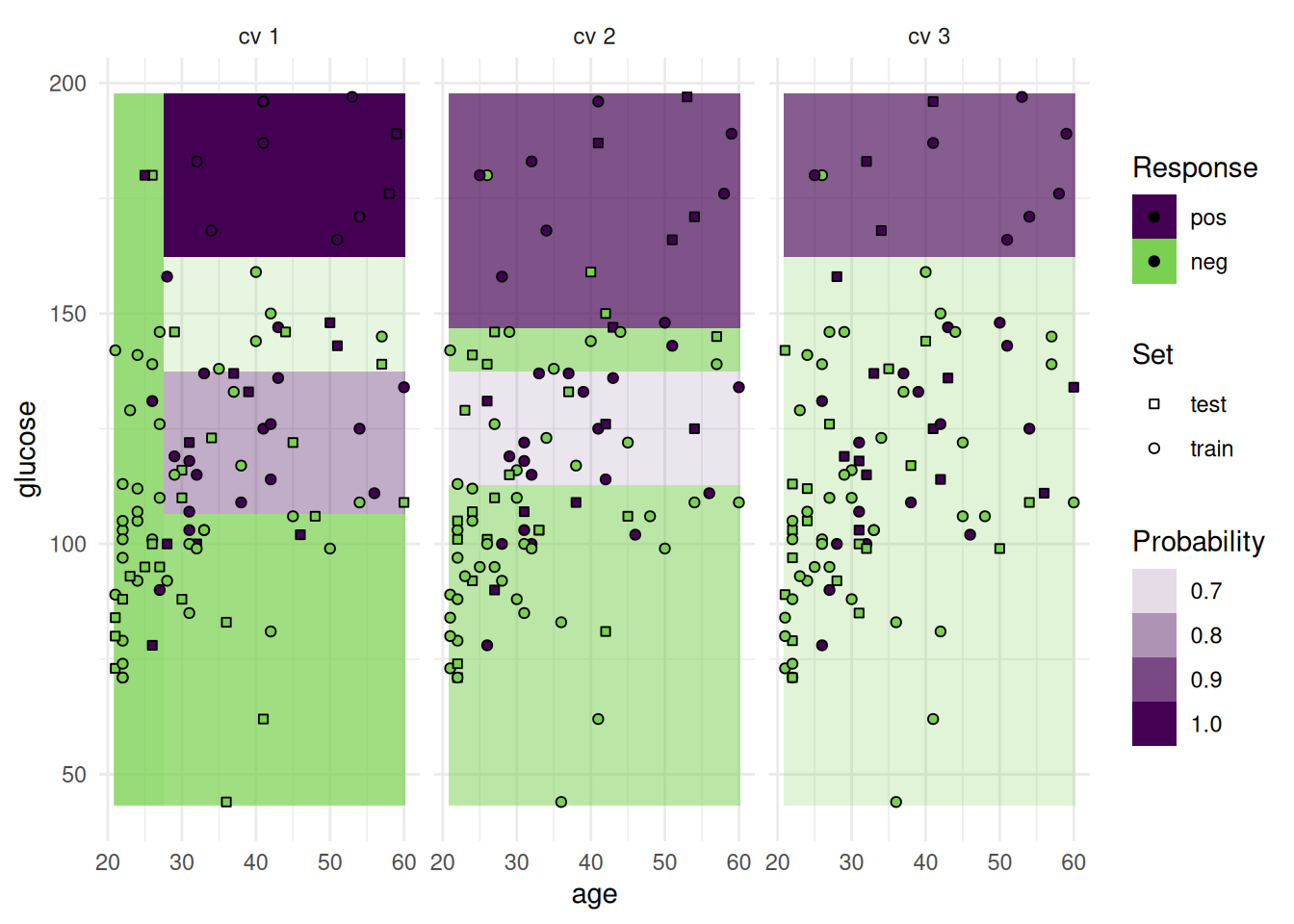
The "prediction" plot can also show categorical features.
task = tsk("german_credit")
task$filter(seq(100))
task$select(c("housing", "employment_duration"))
learner = lrn("classif.rpart")
resampling = rsmp("cv", folds = 3)
rr = resample(task, learner, resampling, store_models = TRUE)

autoplot(rr, type = "prediction")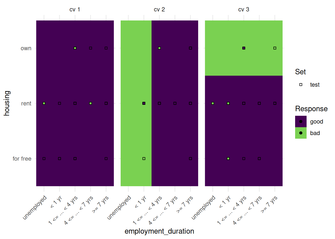
The “prediction” plot shows one feature and the response. Points mark the observations of the test set.
task = tsk("california_housing")
task$select("median_income")
task$filter(seq(100))
learner = lrn("regr.rpart")
resampling = rsmp("cv", folds  = 3)
rr = resample(task, learner, resampling, store_models = TRUE)

autoplot(rr, type = "prediction")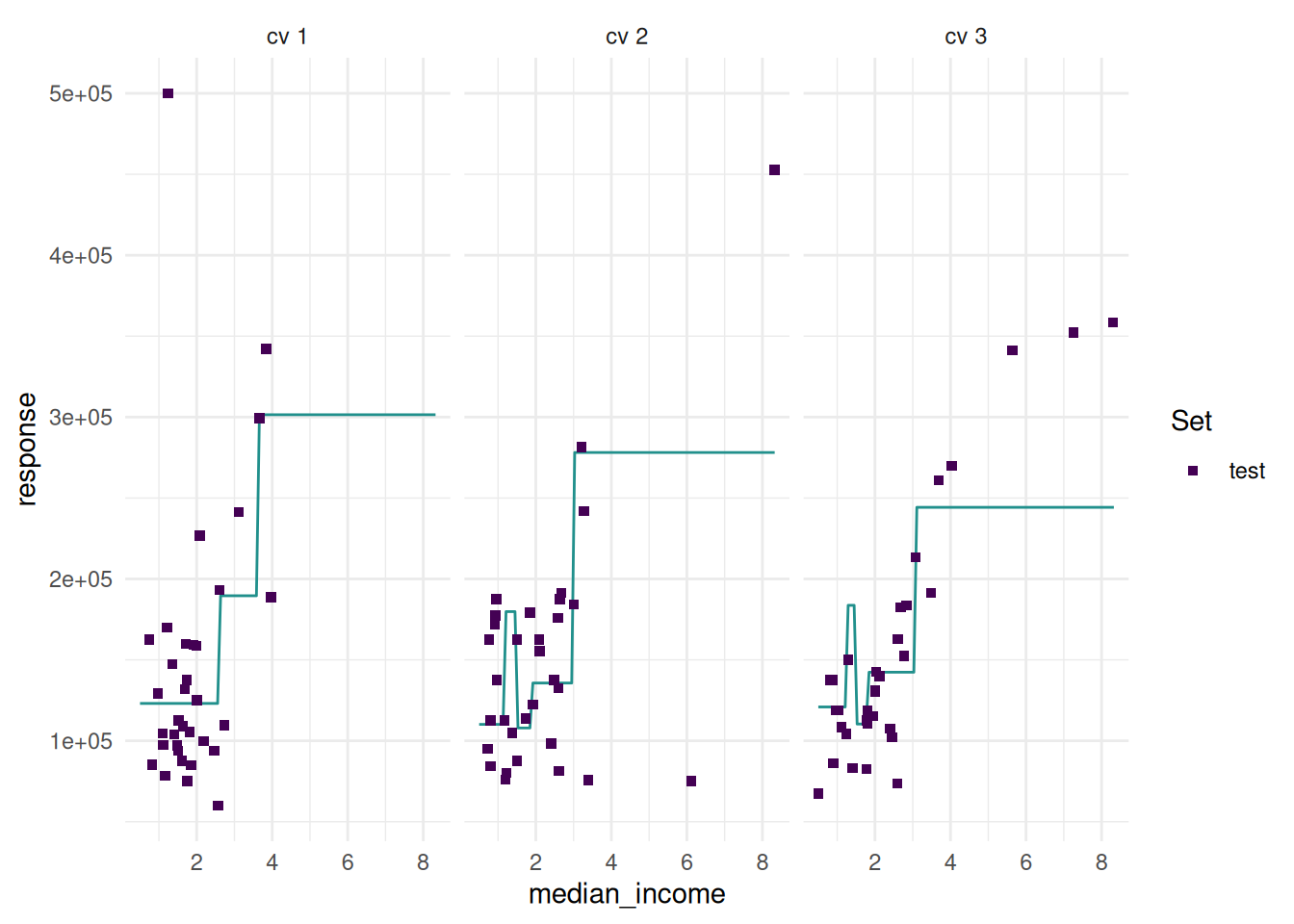
Additionally, we can add confidence bounds.
task = tsk("california_housing")
task$select("median_income")
task$filter(seq(100))
learner = lrn("regr.lm", predict_type = "se")
resampling = rsmp("cv", folds  = 3)
rr = resample(task, learner, resampling, store_models = TRUE)

autoplot(rr, type = "prediction")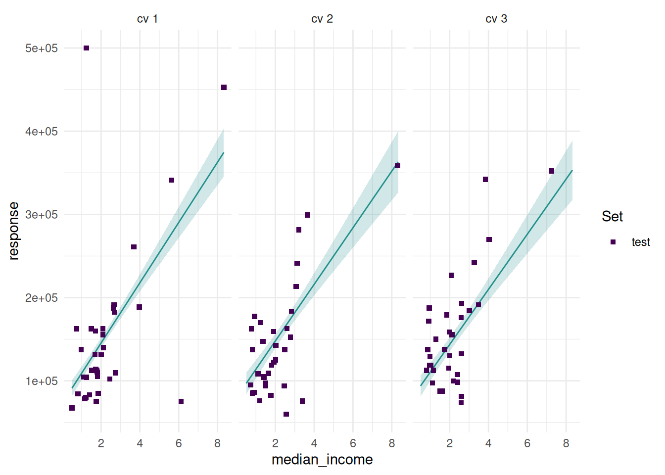
And add the train set.
task = tsk("california_housing")
task$select("median_income")
task$filter(seq(100))
learner = lrn("regr.lm", predict_type = "se", predict_sets = c("train", "test"))
resampling = rsmp("cv", folds = 3)
rr = resample(task, learner, resampling, store_models = TRUE)

autoplot(rr, type = "prediction", predict_sets = c("train", "test"))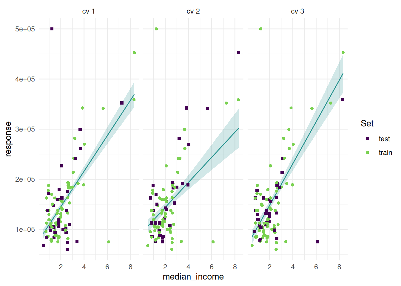
We can also add the prediction surface to the background.
task = tsk("california_housing")
task$select(c("latitude", "longitude"))
task$filter(seq(100))
learner = lrn("regr.rpart")
resampling = rsmp("cv", folds = 3)
rr = resample(task, learner, resampling, store_models = TRUE)

autoplot(rr, type = "prediction")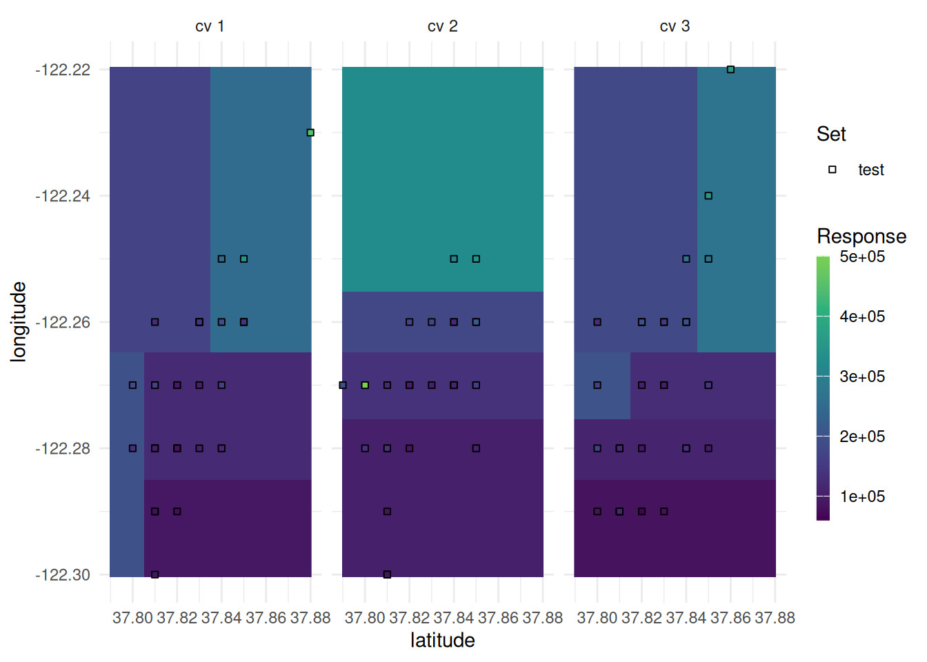
We show the performance distribution of a benchmark with multiple tasks.
tasks = tsks(c("diabetes", "sonar"))
learner = lrns(c("classif.featureless", "classif.rpart", "classif.xgboost"), predict_type = "prob")
resampling = rsmps("cv")
bmr = benchmark(benchmark_grid(tasks, learner, resampling))

autoplot(bmr, type = "boxplot")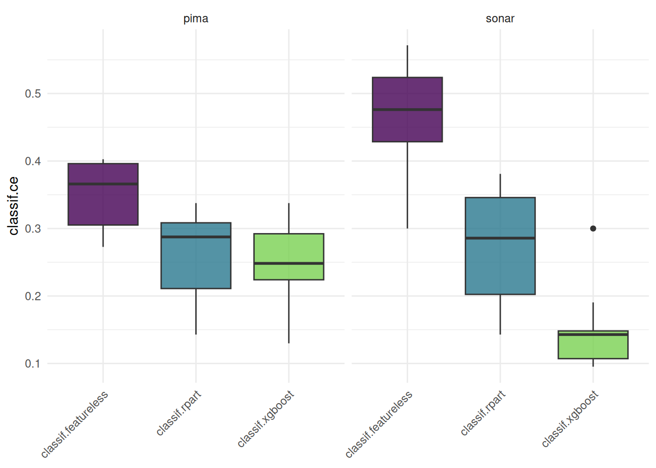
We plot a benchmark result with one task and multiple learners.
tasks = tsk("diabetes")
learner = lrns(c("classif.featureless", "classif.rpart", "classif.xgboost"), predict_type = "prob")
resampling = rsmps("cv")
bmr = benchmark(benchmark_grid(tasks, learner, resampling))
We plot an roc curve for each learner.
autoplot(bmr, type = "roc")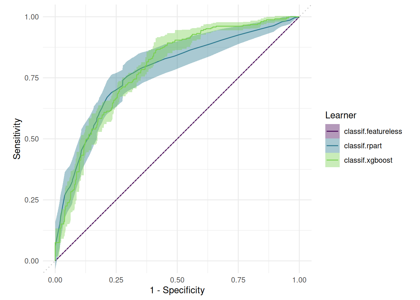
Alternatively, we can plot precision-recall curves.
autoplot(bmr, type = "prc")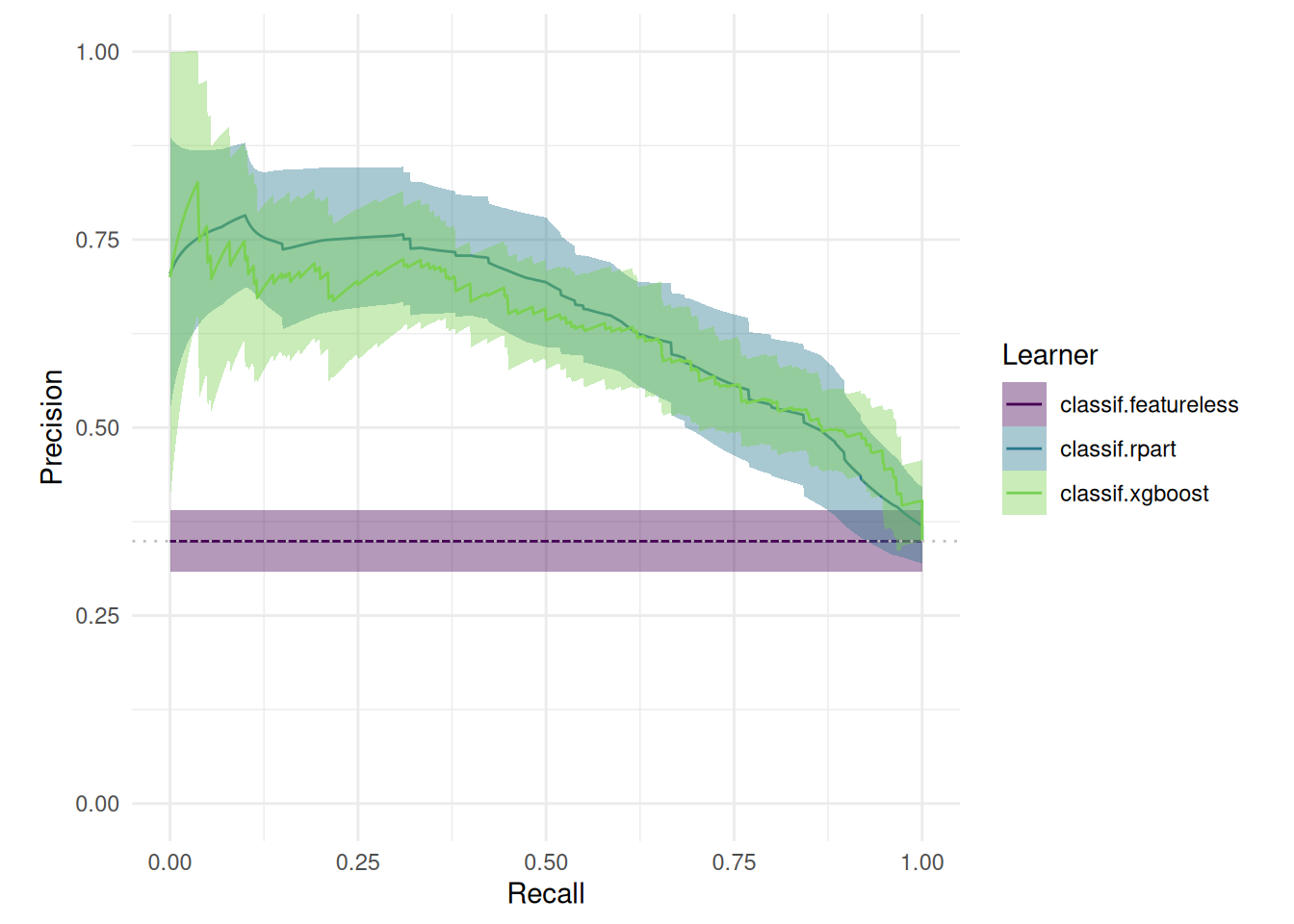
We tune the hyperparameters of a decision tree on the sonar task. The "performance" plot shows the performance over batches.
library(mlr3tuning)
library(mlr3tuningspaces)
library(mlr3learners)

instance = tune(
  tuner = tnr("gensa"),
  task = tsk("sonar"),
  learner = lts(lrn("classif.rpart")),
  resampling = rsmp("holdout"),
  measures = msr("classif.ce"),
  term_evals = 100
)

autoplot(instance, type = "performance")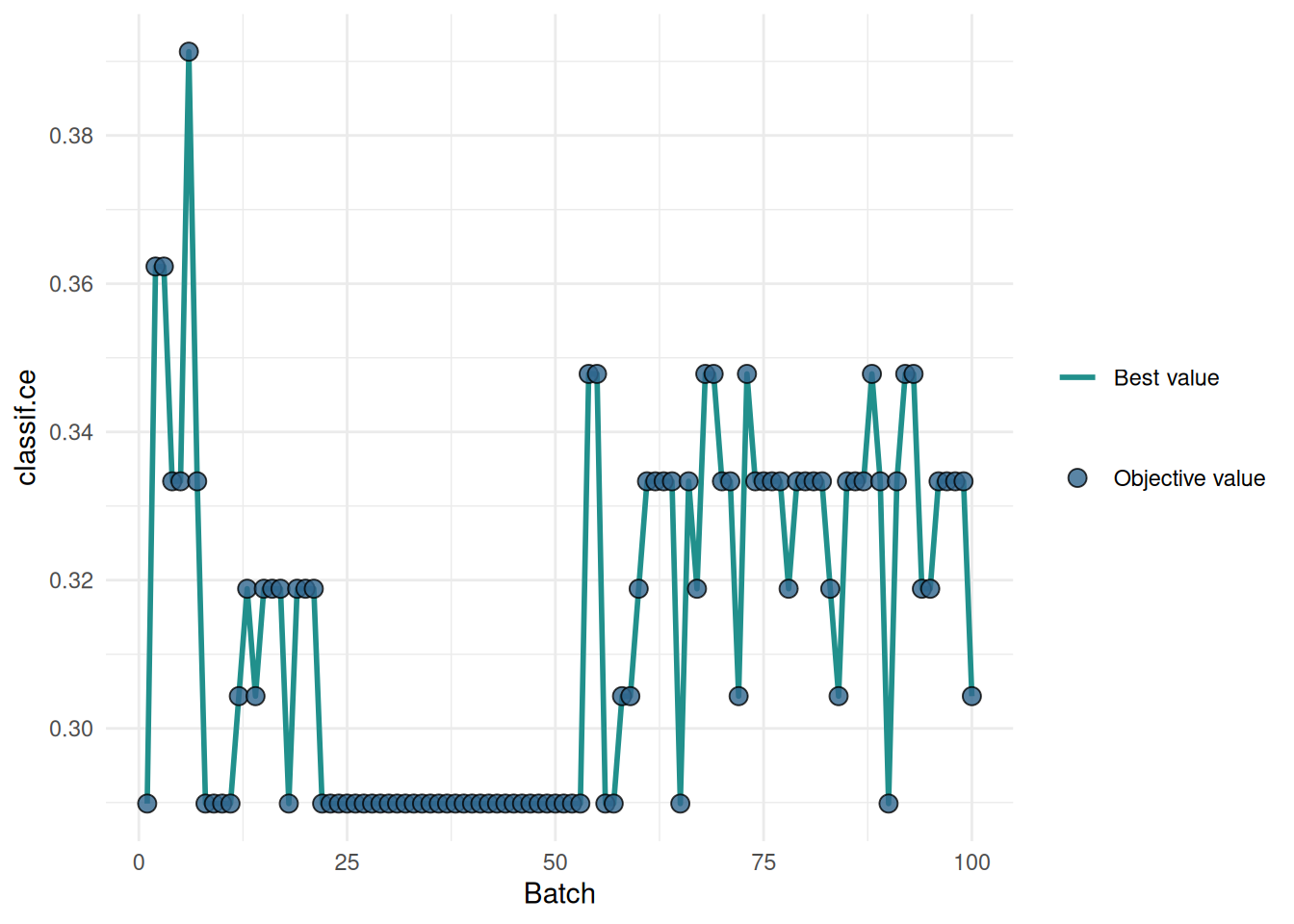
The "incumbent" plot shows the performance of the best hyperparameter setting over the number of evaluations.
autoplot(instance, type = "incumbent")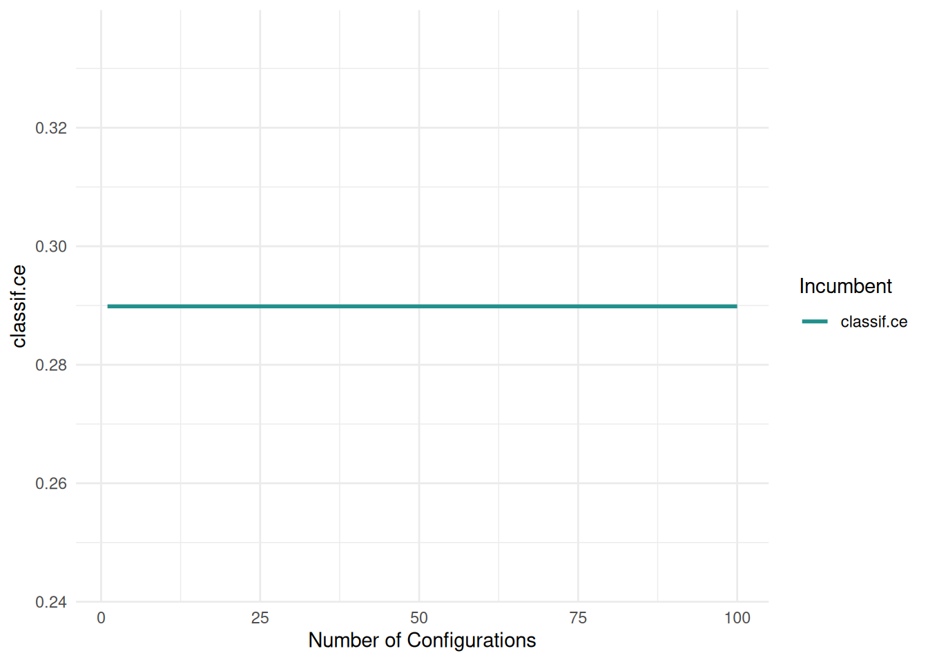
The "parameter" plot shows the performance for each hyperparameter setting.
autoplot(instance, type = "parameter", cols_x = c("cp", "minsplit"))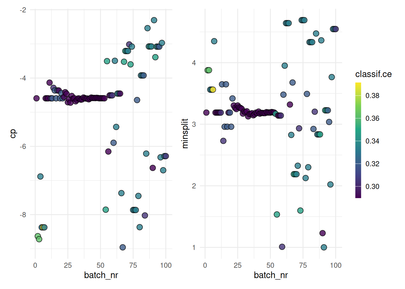
The "marginal" plot shows the performance of different hyperparameter values. The color indicates the batch.
autoplot(instance, type = "marginal", cols_x = "cp")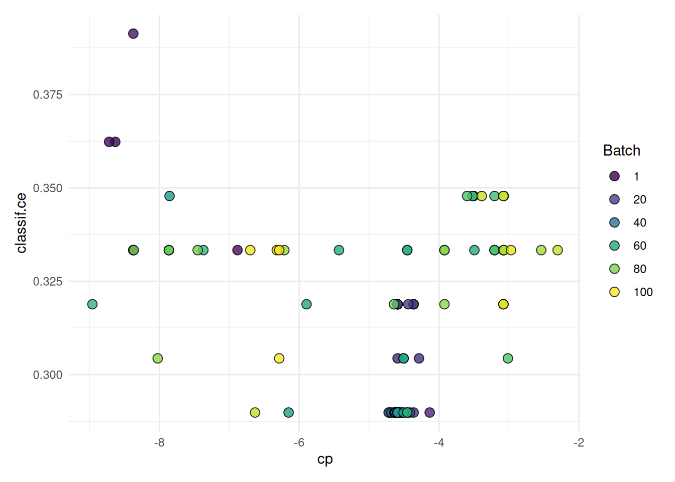
The "parallel" plot visualizes the relationship of hyperparameters.
autoplot(instance, type = "parallel")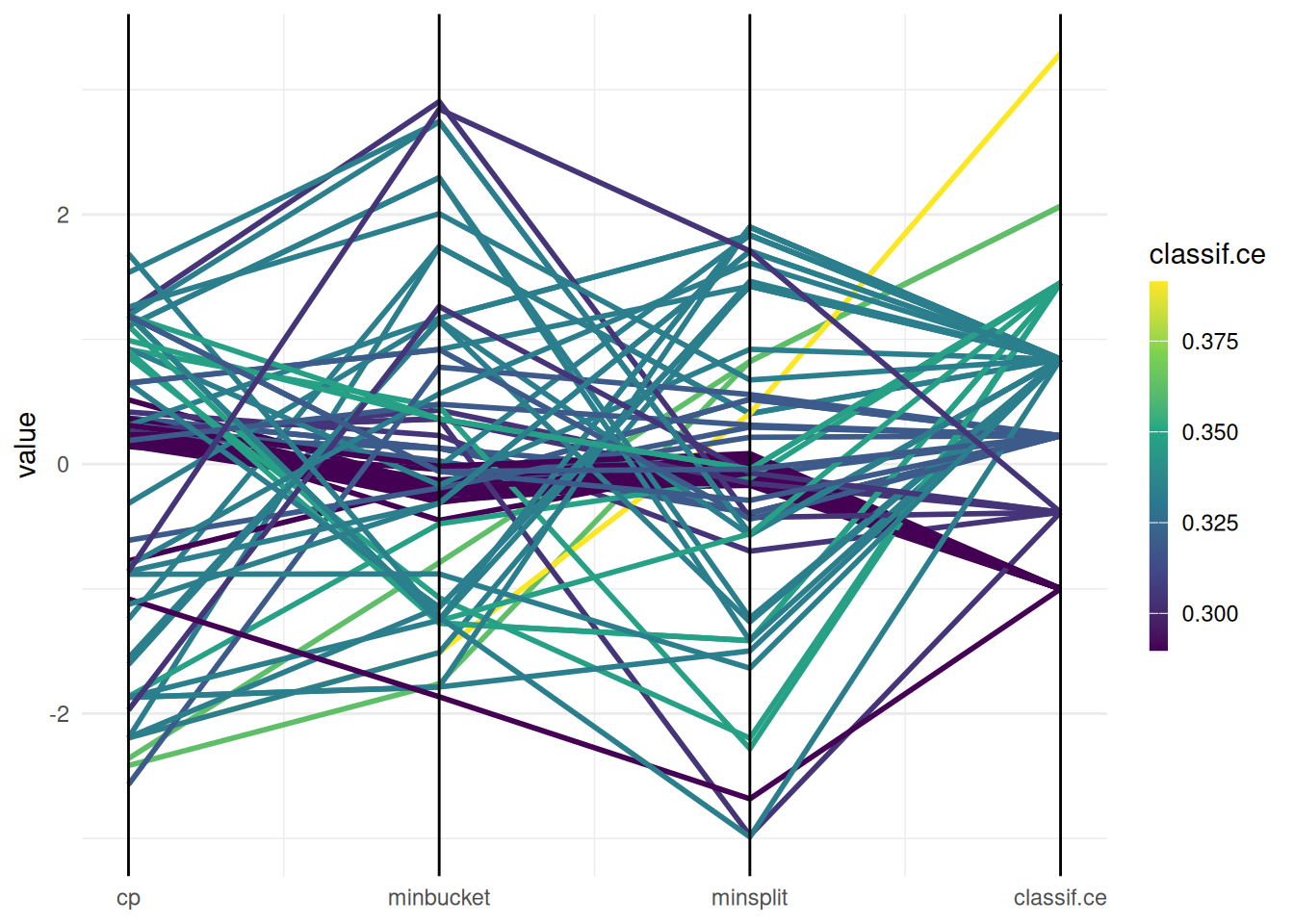
We plot cp against minsplit and color the points by the performance.
autoplot(instance, type = "points", cols_x = c("cp", "minsplit"))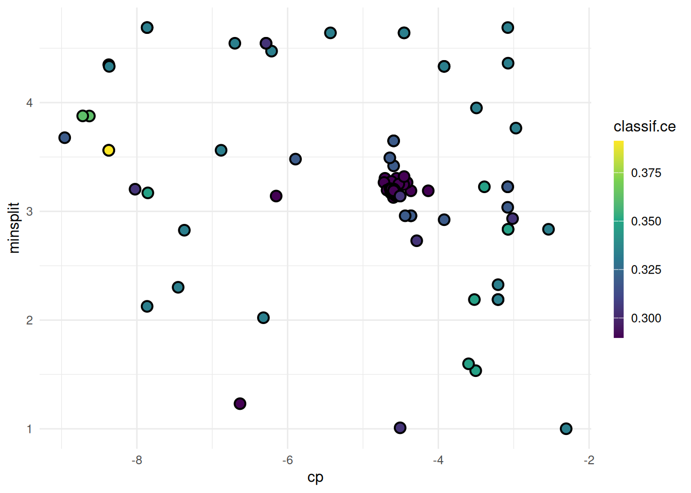
Next, we plot all hyperparameters against each other.
autoplot(instance, type = "pairs")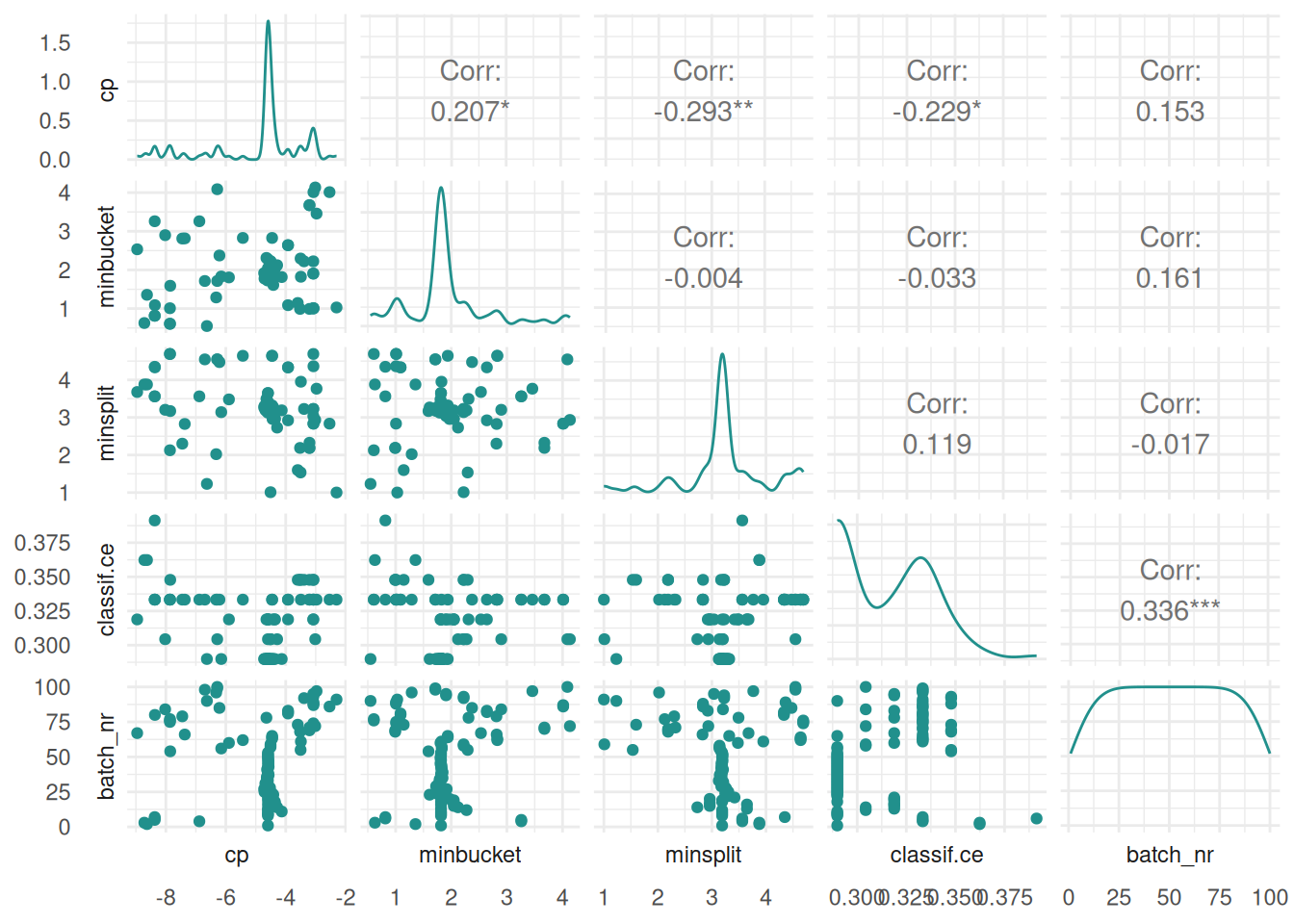
We plot the performance surface of two hyperparameters. The surface is interpolated with a learner.
autoplot(instance, type = "surface", cols_x = c("cp", "minsplit"), learner = mlr3::lrn("regr.ranger"))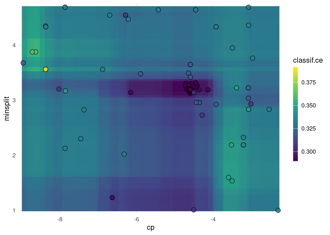
We plot filter scores for the mtcars task.
library(mlr3filters)

task = tsk("mtcars")
f = flt("correlation")
f$calculate(task)

autoplot(f, n = 5)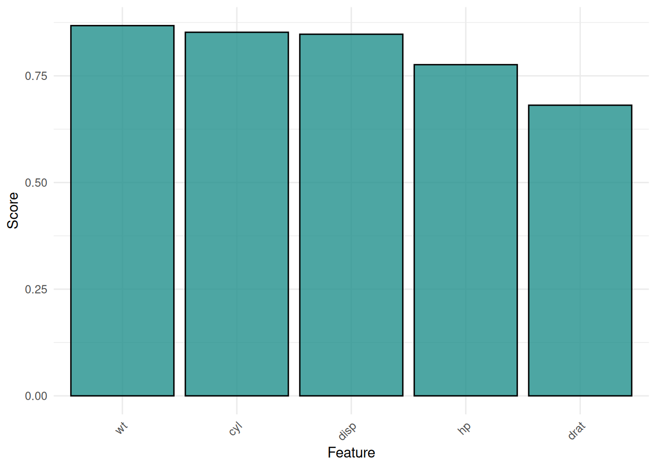
The mlr3viz package brings together the visualization functions of the mlr3 ecosystem. All plots are drawn with the autoplot() function and the appearance can be customized with the theme argument. If you need to highly customize a plot e.g. for a publication, we encourage you to check our code on GitHub. The code should be easily adaptable to your needs. We are also looking forward to new visualizations. You can suggest new plots in an issue on GitHub.
sessioninfo::session_info(info = "packages")═ Session info ═══════════════════════════════════════════════════════════════════════════════════════════════════════
─ Packages ───────────────────────────────────────────────────────────────────────────────────────────────────────────
package * version date (UTC) lib source
assertthat 0.2.1 2019-03-21 [1] RSPM
backports 1.5.1 2026-04-03 [1] RSPM
base64url 1.4 2018-05-14 [1] RSPM
batchtools 0.9.18 2025-08-20 [1] RSPM
bbotk 1.12.0 2026-07-17 [1] RSPM
bit 4.6.0 2025-03-06 [1] RSPM
bit64 4.8.2 2026-05-19 [1] RSPM
brew 1.0-10 2023-12-16 [1] RSPM
callr 3.8.0 2026-06-05 [1] RSPM
checkmate 2.3.4 2026-02-03 [1] RSPM
class 7.3-23 2025-01-01 [2] CRAN (R 4.6.1)
classInt 0.4-11 2025-01-08 [1] RSPM
cli 3.6.6 2026-04-09 [1] RSPM
clue 0.3-68 2026-03-26 [1] RSPM
cluster 2.1.8.2 2026-02-05 [2] CRAN (R 4.6.1)
codetools 0.2-20 2024-03-31 [2] CRAN (R 4.6.1)
coro 1.1.0 2024-11-05 [1] RSPM
crayon 1.5.3 2024-06-20 [1] RSPM
data.table * 1.18.4 2026-05-06 [1] RSPM
DBI 1.3.0 2026-02-25 [1] RSPM
dictionar6 0.1.3 2026-02-23 [1] https://m~
digest 0.6.39 2025-11-19 [1] RSPM
distr6 1.8.4 2026-02-23 [1] https://m~
dplyr 1.2.1 2026-04-03 [1] RSPM
e1071 1.7-17 2025-12-18 [1] RSPM
evaluate 1.0.5 2025-08-27 [1] RSPM
farver 2.1.2 2024-05-13 [1] RSPM
fastmap 1.2.0 2024-05-15 [1] RSPM
foreach 1.5.2 2022-02-02 [1] RSPM
Formula 1.2-6 2026-08-03 [1] RSPM
future 1.75.0 2026-07-20 [1] RSPM
future.apply 1.20.2 2026-02-20 [1] RSPM
generics 0.1.4 2025-05-09 [1] RSPM
GenSA 1.1.15 2025-11-26 [1] RSPM
GGally 2.4.0 2025-08-23 [1] RSPM
ggdendro 0.2.0 2024-02-23 [1] RSPM
ggfortify 0.4.19 2025-07-27 [1] RSPM
ggparty 1.0.0.1 2025-07-10 [1] RSPM
ggplot2 4.0.3 2026-04-22 [1] RSPM
ggstats 0.13.0 2026-03-06 [1] RSPM
glmnet 5.0 2026-05-04 [1] RSPM
globals 0.19.1 2026-03-13 [1] RSPM
glue 1.8.1 2026-04-17 [1] RSPM
gridExtra 2.3.1 2026-06-25 [1] RSPM
gtable 0.3.6 2024-10-25 [1] RSPM
hms 1.1.4 2025-10-17 [1] RSPM
htmltools 0.5.9 2025-12-04 [1] RSPM
htmlwidgets 1.6.4 2023-12-06 [1] RSPM
inum 1.0-5 2023-03-09 [1] RSPM
iterators 1.0.14 2022-02-05 [1] RSPM
jsonlite 2.0.0 2025-03-27 [1] RSPM
KernSmooth 2.23-26 2025-01-01 [2] CRAN (R 4.6.1)
knitr 1.51 2025-12-20 [1] RSPM
labeling 0.4.3 2023-08-29 [1] RSPM
lattice 0.22-9 2026-02-09 [2] CRAN (R 4.6.1)
lgr 0.5.2 2026-01-30 [1] RSPM
libcoin 1.0-13 2026-06-04 [1] RSPM
lifecycle 1.0.5 2026-01-08 [1] RSPM
listenv 1.0.0 2026-06-22 [1] RSPM
magrittr 2.0.5 2026-04-04 [1] RSPM
MASS 7.3-65 2025-02-28 [2] CRAN (R 4.6.1)
Matrix 1.7-5 2026-03-21 [2] CRAN (R 4.6.1)
matrixStats 1.5.0 2025-01-07 [1] RSPM
mgcv 1.9-4 2025-11-07 [2] CRAN (R 4.6.1)
mlr3 * 1.7.1.9000 2026-08-07 [1] Github (mlr-org/mlr3@c63e546)
mlr3batchmark 0.2.2 2025-09-04 [1] RSPM
mlr3benchmark 0.1.7-9000 2026-08-07 [1] Github (mlr-org/mlr3benchmark@771107a)
mlr3cluster * 0.4.1 2026-07-10 [1] RSPM
mlr3cmprsk 0.0.5 2026-04-11 [1] https://m~
mlr3data * 0.9.0 2024-11-08 [1] RSPM
mlr3db 0.7.2 2026-05-22 [1] RSPM
mlr3extralearners 1.6.0 2026-07-14 [1] https://m~
mlr3fairness 0.4.0 2026-08-07 [1] Github (mlr-org/mlr3fairness@6946cbe)
mlr3fda 0.7.1 2026-07-15 [1] RSPM
mlr3filters * 0.9.1 2026-04-23 [1] RSPM
mlr3fselect 1.6.0.9000 2026-08-07 [1] Github (mlr-org/mlr3fselect@3bc9771)
mlr3hyperband 1.1.1 2026-07-25 [1] RSPM
mlr3inferr 0.2.1 2025-11-26 [1] RSPM
mlr3learners * 0.15.1 2026-07-25 [1] RSPM
mlr3mbo 1.2.1 2026-07-26 [1] RSPM
mlr3measures 1.3.0 2026-04-17 [1] RSPM
mlr3misc 0.22.0 2026-06-10 [1] RSPM
mlr3oml 0.12.0 2026-01-28 [1] RSPM
mlr3pipelines 0.11.0-9000 2026-08-07 [1] Github (mlr-org/mlr3pipelines@3a48115)
mlr3proba 0.8.10 2026-06-05 [1] https://m~
mlr3spatial 0.7.0 2026-07-14 [1] RSPM
mlr3spatiotempcv 2.3.5 2026-08-03 [1] RSPM
mlr3torch 0.3.3 2026-01-31 [1] RSPM
mlr3tuning * 1.6.1 2026-07-26 [1] RSPM
mlr3tuningspaces * 0.7.0 2026-07-25 [1] RSPM
mlr3verse 0.3.2 2026-06-22 [1] RSPM
mlr3viz * 0.11.1 2026-07-26 [1] RSPM
mlr3website * 0.0.0.9000 2026-08-07 [1] Github (mlr-org/mlr3website@83dce5a)
moocore 0.3.2 2026-07-12 [1] RSPM
mvtnorm 1.4-2 2026-07-12 [1] RSPM
nlme 3.1-169 2026-03-27 [2] CRAN (R 4.6.1)
ooplah 0.2.0 2022-03-25 [1] https://m~
otel 0.2.0 2025-08-29 [1] RSPM
palmerpenguins 0.1.1 2022-08-15 [1] RSPM
paradox * 1.0.1 2024-07-09 [1] RSPM
parallelly 1.48.0 2026-06-29 [1] RSPM
param6 0.2.4 2026-02-23 [1] https://m~
partykit 1.2-29 2026-07-17 [1] RSPM
patchwork 1.3.2 2025-08-25 [1] RSPM
pillar 1.11.1 2025-09-17 [1] RSPM
pkgconfig 2.0.3 2019-09-22 [1] RSPM
precrec 0.14.5 2025-05-15 [1] RSPM
prettyunits 1.2.0 2023-09-24 [1] RSPM
processx 3.9.0 2026-04-22 [1] RSPM
progress 1.2.3 2023-12-06 [1] RSPM
proxy 0.4-29 2025-12-29 [1] RSPM
ps 1.9.3 2026-04-20 [1] RSPM
purrr 1.2.2 2026-04-10 [1] RSPM
R6 2.6.1 2025-02-15 [1] RSPM
ranger 0.18.0 2026-01-16 [1] RSPM
rappdirs 0.3.4 2026-01-17 [1] RSPM
rbibutils 2.4.1 2026-01-21 [1] RSPM
RColorBrewer 1.1-3 2022-04-03 [1] RSPM
Rcpp 1.1.2 2026-07-05 [1] RSPM
Rdpack 2.6.6 2026-02-08 [1] RSPM
rlang 1.3.0 2026-07-05 [1] RSPM
rmarkdown 2.31 2026-03-26 [1] RSPM
rpart 4.1.27 2026-03-27 [2] CRAN (R 4.6.1)
S7 0.2.2 2026-04-22 [1] RSPM
scales 1.4.0 2025-04-24 [1] RSPM
sessioninfo 1.2.4 2026-06-04 [1] RSPM
set6 0.2.6 2026-02-23 [1] https://m~
sf 1.1-2 2026-07-23 [1] RSPM
shape 1.4.6.1 2024-02-23 [1] RSPM
spacefillr 0.4.0 2025-02-24 [1] RSPM
stringi 1.8.9 2026-08-04 [1] RSPM
stringr 1.6.0 2025-11-04 [1] RSPM
survival 3.8-6 2026-01-16 [2] CRAN (R 4.6.1)
terra 1.9-34 2026-06-19 [1] RSPM
tf 0.5.0 2026-07-14 [1] RSPM
tibble 3.3.1 2026-01-11 [1] RSPM
tidyr 1.3.2 2025-12-19 [1] RSPM
tidyselect 1.2.1 2024-03-11 [1] RSPM
torch 0.17.0 2026-04-11 [1] RSPM
units 1.0-1 2026-03-11 [1] RSPM
uuid 1.2-2 2026-01-23 [1] RSPM
vctrs 0.7.3 2026-04-11 [1] RSPM
viridis 0.6.5 2024-01-29 [1] RSPM
viridisLite 0.4.3 2026-02-04 [1] RSPM
withr 3.0.3 2026-06-19 [1] RSPM
xfun 0.60 2026-07-09 [1] RSPM
xgboost 3.2.1.1 2026-03-18 [1] CRAN (R 4.6.1)
yaml 2.3.12 2025-12-10 [1] RSPM
zoo 1.9-0 2026-07-31 [1] RSPM
[1] /usr/local/lib/R/site-library
[2] /usr/local/lib/R/library
* ── Packages attached to the search path.
──────────────────────────────────────────────────────────────────────────────────────────────────────────────────────